We have already encountered the position vector $\mathbf{R}$, also known as the radius vector, which points from an arbitrary fixed origin $O$ to each point in the Euclidean space. The purpose of the position vector is, of course, to represent the position of the corresponding point by an object that is subject to analytical operations. Every one of our geometric analyses will start with the position vector. However, despite its fundamental role, it will rarely figure explicitly in advanced stages of most of our analyses, as we will be more interested in its derivatives rather than the position vector itself. This is part of the reason why the origin $O$ can be selected arbitrarily: its location has no bearing on the derivatives of $\mathbf{R}$.

The position vector is a vector field, since to every point in space, there corresponds a particular value of $\mathbf{R}$. However, as you see from the above figure, it is usually depicted in an unusual way compared to most vector fields. For most vector fields, such as the velocity distribution of a fluid, we usually imagine vectors emanating from the associated points in the Euclidean space, as in the following figure from Chapter 4. The position vector, on the other hand, is best imagined emanating from the origin $O$, as you see in the preceding figure. Because of this unconventional representation, we need to remind ourselves that the position vector is associated with the point to which it is pointing, rather than the origin.

Now, impose a coordinate system upon the Euclidean space. Assume that the Euclidean space is three-dimensional and, as usual, denote the coordinates by $Z^{1}$, $Z^{2}$, and $Z^{3}$ or, collectively, $Z^{i}$. Importantly, the coordinate system is assumed to be completely arbitrary as long as it is sufficiently smooth in the sense described below. If the coordinate system has the concept of the coordinate origin -- as most of the standard coordinate systems do -- it need not coincide with the origin $O$ that anchors the position vector field $\mathbf{R}$. We also remind the reader that the decision to use a superscript to enumerate the coordinates is completely arbitrary in its own right. However, once the decision to use a superscript to enumerate the coordinates is made, the placement of indices on all subsequent objects is uniquely prescribed by the rules of the tensor notation.

In the absence of a coordinate system, the position vector is described by the term field rather than function. A field is an association between the points of a Euclidean space and some quantity. As such, the position vector is an example of a vector field. Meanwhile, the temperature distribution in a room is an example of a scalar field. The term function, on the other hand, describes an association between sets of numbers and some quantity. Thus, with a coordinate system imposed upon the Euclidean space, we may begin to speak of the position vector function This function maps triplets of numbers $Z^{1},Z^{2},Z^{3}$ to the value of the position vector $\mathbf{R}$ at the point with coordinates $Z^{1}$, $Z^{2}$, and $Z^{3}$.

By smoothness of the coordinate system we understand the differentiability characteristics of the function $\mathbf{R}\left( Z^{1},Z^{2},Z^{3}\right)$. For most analyses, existence of second derivatives is sufficient. We will often describe $\mathbf{R}\left( Z^{1},Z^{2},Z^{3}\right)$ as sufficiently smooth, meaning that as many derivatives are available as required by the analysis at hand.

As we have similarly noted in a number of analogous contexts, the symbol $\mathbf{R}$ in the expression $\mathbf{R}\left( Z^{1},Z^{2},Z^{3}\right)$ is being used in a new capacity compared to the symbol $\mathbf{R}$ in the absence of coordinates. In the absence of coordinates, $\mathbf{R}$ denotes a vector field, i.e. an association between points and vectors. In the expression $\mathbf{R}\left( Z^{1},Z^{2},Z^{3}\right)$, however, $\mathbf{R}$ denotes a vector-valued function of the three independent variables $Z^{1}$, $Z^{2}$, and $Z^{3}$. This is another example of assigning the same symbol two closely related, albeit different, meanings.

From this point forward, we will collapse the functional arguments of all functions of coordinates into the symbol $Z$. For example, the function $\mathbf{R}\left( Z^{1},Z^{2},Z^{3}\right)$ will be denoted by the symbol In addition to its compactness, the symbol $\mathbf{R}\left( Z\right)$ has the advantage that it works in any number of dimensions. The alternative symbol $\mathbf{R}\left( Z^{i}\right)$ cannot be used since it makes the index $i$ appear live and leaves it hanging, which violates the rules of the tensor notation.

The function $\mathbf{R}\left( Z\right)$ is the starting point for a crucial sequence of definitions. Before we turn our attention to those definitions, it is important to reiterate that the position vector $\mathbf{R}$ is a primary object that is to be understood and accepted on its own geometric terms. It is counterproductive to imagine some a priori basis with respect to which $\mathbf{R}$ could be represented by its components. There is simply no such basis available -- nor is one needed.

The remainder of the objects introduced in this Chapter are denoted by symbols anchored by the letter $Z$. This includes the covariant basis $\mathbf{Z}_{i}$, the covariant metric tensor $Z_{ij}$, the volume element $\sqrt{Z}$, the contravariant metric tensor $Z^{ij}$, and the contravariant basis $\mathbf{Z}^{i}$. Despite the fact that the same letter is used in each of these symbols, they can be easily distinguished by their indicial signatures. Additionally, the symbol $\mathbf{Z}^{i}$ for the contravariant basis is distinguished from the symbol $Z^{i}$ denoting the coordinates by the fact that the letter $Z$ is textbf{bold} in the former and plain in the latter.

The covariant basis $\mathbf{Z}_{1}$, $\mathbf{Z}_{2}$, $\mathbf{Z}_{3}$ -- or, collectively, $\mathbf{Z}_{i}$ -- is a generalization of the affine coordinate basis $\mathbf{i}$, $\mathbf{j}$, $\mathbf{k}$ to curvilinear coordinates. It is constructed from the position vector $\mathbf{R}\left( Z\right)$ by differentiation with respect to each of the coordinates, i.e. Of course, the vectors $\mathbf{Z}_{1}$, $\mathbf{Z}_{2}$, and $\mathbf{Z} _{3}$ constitute a legitimate basis only when they form a linearly independent set. Points where this is not the case are called singular and almost always require special treatment.

As we have already discussed on several occasions, the term covariant describes the placement of the index as a subscript and, correspondingly, the manner in which the basis $\mathbf{Z}_{i}$ transforms under a coordinates transformation. For the time being, we will use the term covariant without exploring its deeper meaning. Also note that, in reference to $\mathbf{Z}_{i}$, we will frequently drop the term covariant and refer to $\mathbf{Z}_{i}$ simply as the basis.

It is not surprising that the first new fundamental object in a Euclidean space is introduced by means of partial differentiation with respect to the coordinates $Z^{i}$. After all, it is just about the only interesting operation that we have at our disposal that can be applied to $\mathbf{R} \left( Z\right)$. Furthermore, it is remarkable that the generalization of the coordinate basis from affine to general coordinates is accomplished by such a simple operation. Just like that, we are able to decompose vectors, and thus conduct component analysis, in general coordinate systems. Keep in mind, however, that -- unlike the coordinate basis $\mathbf{i}$, $\mathbf{j}$, $\mathbf{k}$ in affine coordinates -- the covariant basis $\mathbf{Z}_{i}$ varies from one point to another and therefore the component space is specific to each point in space. As a result, we must imagine an independent linear space at each point and work out how each space interacts with the neighboring spaces. In the near future, we will have a lot to say about this.

Since we have decided to represent the function $\mathbf{R}\left( Z^{1} ,Z^{2},Z^{3}\right)$ by the symbol $\mathbf{R}\left( Z\right)$, the definition of the covariant basis can be expressed by the more compact equations With the help of the tensor notation, the above definitions can be combined into a single indicial equation, i.e.

The fact that the covariant basis ends up with a subscript illustrates an important feature of the tensor notation which we have mentioned earlier on a number of occasions. Namely, that by strongly suggesting the proper placements of indices, the tensor notation tends to predict the manner in which objects transform under coordinate transformations. For the covariant basis $\mathbf{Z}_{i}$, the subscript is a natural choice since, as we discussed in Chapter 7, in the expression the index $i$ appears as a superscript in the "denominator". Thus, the tensor notation predicts that the covariant basis transforms in a manner opposite of the coordinates. In Chapter 6, we have already observed that this is the case for transformations between affine coordinates. For general coordinate transformations, this will be confirmed in Chapter 14.

The covariant basis $\mathbf{Z}_{i}$ is used for the decomposition of vectors at a given point. When a vector $\mathbf{U}$ is decomposed with respect to $\mathbf{Z}_{i}$, the resulting coefficients are naturally assigned superscripts, i.e. in order to utilize the summation conventions in the equation The components $U^{i}$ of a vector $\mathbf{U}$ with respect to the covariant basis $\mathbf{Z}_{i}$ are referred to as the contravariant components. Of course, the broad goal of our analysis is to replace vectors with their components so that we are able to solve problems by analytical rather than geometric means. Thus, a detailed discussion of the components of vectors and their use will be postponed until the next Chapter devoted entirely to coordinate space analysis.

Finally, note that it is not advisable to decompose the elements of the basis $\mathbf{Z}_{i}$ itself with respect to some a priori supplementary basis. Given the prevalent use of Cartesian coordinates, the temptation may be great to think of each vector $\mathbf{Z}_{i}$ as a triplet of numbers with respect to some background Cartesian basis $\mathbf{i}$, $\mathbf{j}$, $\mathbf{k}$. However, this would obscure the primary decompositional role of the covariant basis. The covariant basis $\mathbf{Z}_{i}$ is used for decomposing other vectors but itself need not be decomposed. The buck, so to say, stops with $\mathbf{Z}_{i}$.

The primary geometric characteristic of the vectors $\mathbf{Z}_{i}$ is that they are tangential to the corresponding coordinate lines. To see why this is so for, say,textbf{ }$\mathbf{Z}_{1}$, consider the function (Note that we are now using the letter $\mathbf{R}$ to denote yet another function, this time of one variable $\gamma$.) The vectors $\mathbf{R}\left( \gamma\right)$ trace out the coordinate line corresponding to $Z^{1}$. Therefore, as we studied in Chapter 5, the derivative is tangential to that coordinate line. Of course, since $\mathbf{R}^{\prime }\left( \gamma\right)$ is the same as we conclude that the vector $\mathbf{Z}_{1}$ is tangential to the coordinate line corresponding to $Z^{1}$, as we set out to show.

The covariant basis is particularly easy to visualize when the coordinate lines are drawn at integer increments, as in the following two-dimensional figure. In the context of such a representation, the approximate length of $\mathbf{Z}_{i}$ at a node is such that its tip is located in the vicinity of the neighboring node whose coordinate $Z^{i}$ exceeds that of its tail by $h=1$. For example, the tip of the vector $\mathbf{Z}_{1}$ at the point with coordinates $\left( Z^{1},Z^{2},Z^{3}\right)$ falls near the point with coordinates $\left( Z^{1}+1,Z^{2},Z^{3}\right)$. This is so because, in the limit the "intermediate" vector corresponding to the finite value $h=1$ falls exactly at the point with coordinates $\left( Z^{1}+1,Z^{2} ,Z^{3}\right)$ and, in the limit as $h$ approaches $0$, it ought to be approximately so.

For general curvilinear coordinate systems, the covariant basis varies from one point to another. In an affine coordinate system, thanks to its regularity, the covariant basis is the same at all points and coincides with the coordinate basis $\mathbf{i}$, $\mathbf{j}$, $\mathbf{k}$. In other words, the basis vector $\mathbf{Z}_{i}$ points from the point with coordinates $\left( Z^{1},Z^{2},Z^{3}\right)$ to the point whose $i$-th coordinate is increased by $1$. For example, $\mathbf{Z}_{2}$ points from the point with coordinates $\left( Z^{1},Z^{2},Z^{3}\right)$ to the point with coordinates $\left( Z^{1},Z^{2}+1,Z^{3}\right)$. In curvilinear coordinates, the preceding statement is approximately true at points where the magnitude of the second derivatives of $\mathbf{R}\left( Z\right)$ is not too great.

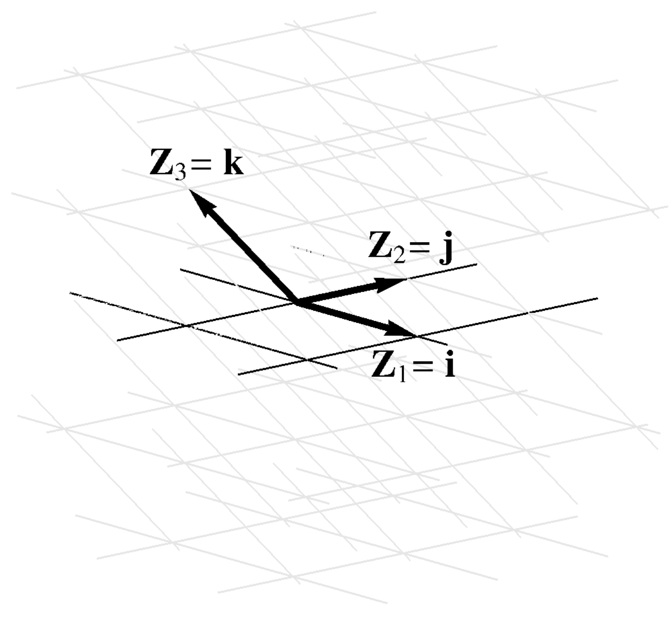
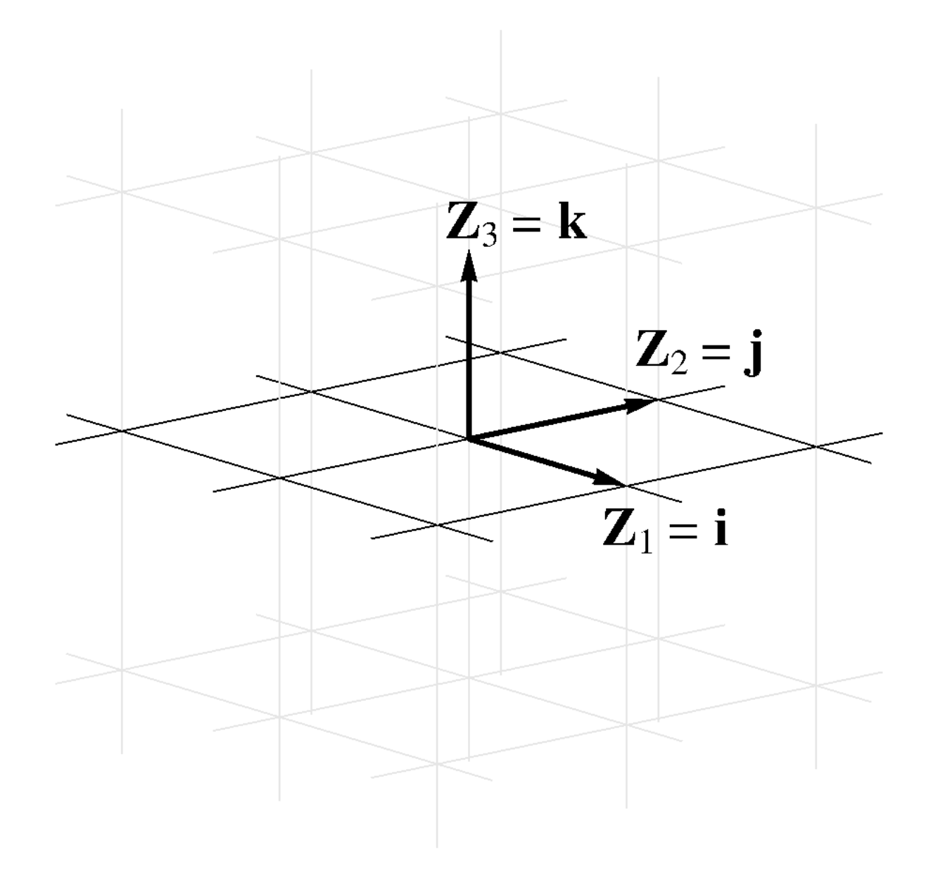
Since Cartesian coordinates are a special case of affine coordinates, the Cartesian covariant basis is the same at all points. Cartesian coordinate lines form a regular orthogonal unit grid and therefore the covariant basis consists of orthogonal unit, i.e. orthonormal, vectors. The following figure shows the Cartesian covariant bases in two and three dimensions. In conclusion, the familiar affine basis $\mathbf{i}$, $\mathbf{j}$, $\mathbf{k}$ fits perfectly into the new framework where the coordinate basis is constructed by differentiating the position vector $\mathbf{R}$ with respect to each of the coordinates.

In polar coordinates $r,\theta$, the coordinate $Z^{1}$ corresponds to $r$ and $Z^{2}$ corresponds to $\theta$. The covariant basis vector $\mathbf{Z}_{1}$, given by the equation is a unit vector that points in the radial direction away from the origin $O$. Demonstrating this fact is left as an exercise. The vector $\mathbf{Z}_{2}$ is given by Recall from Section 4.3 that the derivative $\mathbf{R}^{\prime}\left( \gamma\right)$ of the position vector $\mathbf{R}\left( \gamma\right)$ tracing out a circle of radius $r$ is a vector tangential to the circle also of length $r$. Of course, this configuration corresponds exactly to the calculation of $\mathbf{Z}_{2}$. Thus, $\mathbf{Z}_{2}$ is a vector of length $r$ that points in the counterclockwise tangential direction to the coordinate circle. These findings regarding the covariant basis $\mathbf{Z}_{i}$ for polar coordinates are illustrated in the following figure.

Observe that the covariant basis in polar coordinates is orthogonal. Interestingly, in some textbooks, the vector $\mathbf{Z}_{2}$ is scaled to unit length in order to produce an orthonormal basis at every point. This is highly inadvisable due to the numerous disadvantages in exchange for little gain.

Polar coordinates present us with our first example of a coordinate basis that varies from one point to another. This variability is of enormous importance. Some of its most crucial implications are described below in Section 9.2.10 and will be discussed further later in our narrative.

Cylindrical coordinates augment polar coordinates $r,\theta$ with the coordinate $z$ whose coordinate lines are straight lines orthogonal to the coordinate plane. Within each plane parallel to the coordinate plane, i.e. within each coordinate surface corresponding to a constant $z$, the vectors coincide with the covariant basis in polar coordinates. The additional vector $\mathbf{Z}_{3}$, given by is a constant unit vector orthogonal to the coordinate plane that points in the "upward" direction -- in other words, the set $\mathbf{Z}_{1}$, $\mathbf{Z}_{2}$, $\mathbf{Z}_{3}$ is positively oriented. Note that even with the addition of $\mathbf{Z}_{3}$, the covariant basis remains orthogonal.

In order to describe the covariant basis $\mathbf{Z}_{i}$ in spherical coordinates $r,\theta,\varphi$, we will use a combination of words and figures. The first vector is a unit vector that points in the radial direction away from the origin $O$. The second vector corresponds to the rate of change in the position vector $\mathbf{R}$ along a meridian. Thus, $\mathbf{Z}_{2}$ is a vector of length $r$ that points in the direction tangential to the meridian away from the north pole, i.e. the point with $\theta=0$. The third vector corresponds to the rate of change in the position vector $\mathbf{R}$ along a parallel and is thus tangential to that parallel. Since a parallel at colatitude $\theta$ has radius $r\sin\theta$, the length of $\mathbf{Z}_{3}$ is also $r\sin\theta$. The following figure shows the basis vectors $\mathbf{Z}_{2}$ and $\mathbf{Z}_{3}$ on the coordinate sphere of radius $r$. As was the case with cylindrical coordinates, the basis $\mathbf{Z} _{1},\mathbf{Z}_{2},\mathbf{Z}_{3}$ is positively oriented. Furthermore, it is orthogonal but not orthonormal.

As we have pointed out, the covariant bases for Cartesian, polar, cylindrical, and spherical coordinates are orthogonal. Coordinate systems that have this property are themselves known as orthogonal. Since the covariant basis vectors are tangential to the coordinate lines, orthogonal systems can be equivalently characterized by orthogonal coordinate lines. There is no particular significance to orthogonal coordinate systems, except that some calculations are simplified. The following figure shows the coordinate lines for a generic orthogonal system.

You may be wondering whether there exist orthonormal coordinate systems other than Cartesian. The surprising answer is no: as we discuss below in Section 9.3.6, all orthonormal coordinates are necessarily Cartesian.

If you are coming from an exclusively affine background, the implications of the spatial variability of the covariant basis in curvilinear coordinates may require some getting used to. In some ways, the difference is dramatic. For example, the components of one and the same vector calculated at different points are likely to be distinct. Conversely, two vectors with identical components are likely to be distinct. Furthermore, vectors at different points cannot be added together by adding their components. This insight has a number implications, including for integration which, in essence, is a form of addition. Suppose that $g^{i}\left( Z\right)$ represent the components of the gravitational force field per unit mass acting upon a body with density $\rho$ that occupies the domain $\Omega$. If the coordinate system as affine, then the components $F^{i}$ of the total force $\mathbf{F}$ are given by the integral In curvilinear coordinates, on the other hand, the above integral is meaningless since it requires the addition of components of vectors calculated with respect to (an infinity of) different bases.

These difficulties, however, should not in any way dissuade us from utilizing curvilinear coordinates whose use is essential in most situations. Furthermore, in many geometric spaces, such as the surface of a sphere and most other curved surfaces, curvilinear coordinates are the only available option. And even when affine coordinates are feasible, curvilinear coordinates may nevertheless be a natural choice and experience shows that overcoming difficulties that stem from natural choices is always a worthwhile endeavor. Indeed, our future experience will demonstrate that allowing curvilinear coordinates is an unequivocal improvement over the exclusive use of affine coordinates. The additional complexity will prove to be not an obstacle but an impetus for deeper insights that would not have been come form affine analysis.

We have arrived at one of the central objects in our subject: the covariant metric tensor. By definition, the elements of the covariant metric tensor $Z_{ij}$ are the pairwise dot products of the covariant basis vectors $\mathbf{Z}_{i}$, i.e. Since the dot product is commutative, the metric tensor is symmetric, i.e. and can be organized into a symmetric $3\times3$ matrix This matrix is entirely analogous to the dot product matrix from Chapter 2.

The central role of the covariant metric tensor is to facilitate the calculation of dot products -- and thus of lengths and angles -- in the coordinate space. In the next Chapter, we will show that the dot product $\mathbf{U}\cdot\mathbf{V}$ of vectors with components $U^{i}$ and $V^{i}$ is given by Thus, the term metric refers to covariant metric tensor's role in representing geometric measurements.

A few sections below, we will introduce the contravariant metric tensor $Z^{ij}$ as the matrix inverse of the covariant metric tensor $Z_{ij}$. Because it will almost always be clear from the context which of the two objects we are referring to, the adjectives covariant and contravariant are often dropped and the shorter term metric tensor is used to describe both tensors. The terms fundamental tensor and fundamental form can also be used to describe both metric tensors.

When we write the covariant basis directly in terms of the position vector $\mathbf{R}$, i.e. we see the entire scope of its construction from the position vector which we chose as the starting point of our analysis. The recipe requires the ability to measure distances and angles (which go into the dot product), as well as the ability to differentiate vector-valued functions with respect to the coordinates. However, once the metric tensor $Z_{ij}$ is calculated, it can be used to calculate the dot product, and therefore distances and angles, in the component space by analytical means. Furthermore, as we will soon discover, the metric tensor plays a crucial role in the component space differentiation of vector-valued functions, again by analytical means. These abservations suggest the possibility of an entirely new approach to the subject of Geometry where the metric tensor -- rather than lengths and angles -- serves as the starting point. The fundamentals of this approach, known as Riemannian Geometry, will be outlined in Chapter 20.

In affine coordinates, the covariant basis $\mathbf{Z}_{i}$ is the same at all points and, therefore, so is the metric tensor $Z_{ij}$. Using the symbols $\mathbf{i}$, $\mathbf{j}$, and $\mathbf{k}$ to denote the elements of the covariant basis, the metric tensor $Z_{ij}$ correspond to the constant matrix

For a specific two-dimensional example, consider the affine coordinate system illustrated in the following figure, where the length of $\mathbf{i}$ is $1$, the length of $\mathbf{j}$ is $2$, and the angle between $\mathbf{i}$ and $\mathbf{j}$ is $\pi/3$. Then

In Cartesian coordinates, the covariant basis $\mathbf{i,j,k}$ is orthonormal and, therefore, $Z_{ij}$ corresponds to the identity matrix Generally speaking, in an $n$-dimensional Euclidean space, the elements of the Cartesian metric tensor can be captured by the equation Note that we are careful not to use the Kronecker delta symbol $\delta_{j}^{i}$ on the right since its indicial signature does not match that of $Z_{ij}$ and therefore the equation $Z_{ij}=\delta_{j}^{i}$ would have been invalid from the tensor notation point of view. That said, once we introduce index juggling in Chapter 11, we will establish a surprising equivalence between the metric tensor and the Kronecker delta symbol.

Recall that the covariant basis in polar coordinates consists of two orthogonal vectors $\mathbf{Z}_{1}$ and $\mathbf{Z}_{2}$ of lengths $1$ and $r$. Therefore, the covariant metric tensor $Z_{ij}$ has two nonzero elements Thus, The diagonal property of the resulting matrix reflects the orthogonality of the coordinate system.

It is interesting to note that the elements of $Z_{ij}$ have varying "units" of length. If meter is used as the unit of length in the Euclidean space, then $Z_{11}$ is dimensionless while $Z_{22}$ is measured in square meters. The units of the off-diagonal zero entries are meters. While the issue of units is quite subtle, we will be able to side step it completely throughout our narrative.

Since the cylindrical covariant basis consists of orthogonal vectors $\mathbf{Z}_{1}$, $\mathbf{Z}_{2}$ and $\mathbf{Z}_{3}$ of lengths $1$, $r$, and $1$,

Based on the above description of the covariant basis $\mathbf{Z}_{i}$ in spherical coordinates, it is an entirely straightforward matter to show that in spherical coordinates,

Two different coordinate systems related by a rigid transformation, i.e. a combination of rotation, reflection, and translation, produce the same covariant metric tensor function $Z_{ij}\left( Z\right)$. For example, the following figure shows a rotation of a coordinate system by an angle $\alpha$ followed by translation by a vector $\mathbf{d}$. It is clear that $Z_{ij}\left( Z\right)$ is unchanged under this transformation since the relative arrangement of the covariant basis vectors is exactly the same at corresponding points.

Interestingly, the converse is also true: if two coordinate systems are characterized by the same covariant basis function $Z_{ij}\left( Z\right)$ then they are necessarily related by a rigid transformation. This statement is the object of Problem 9.1 at the end of this Chapter. This observation shows that the covariant metric tensor $Z_{ij}$ retains a great deal of information about the coordinate system. In fact, it retains all the information, except its absolute location and orientation (in the sense of rotation and reflection).

In particular, if the elements of the metric tensor $Z_{ij}$ form the identity matrix, then the coordinate system is necessarily Cartesian. In other words, all orthonormal coordinates are Cartesian. In other words, there cannot exist a coordinate system, such as the one "illustrated" in the following figure, where the covariant basis $\mathbf{Z}_{i}$ is orthonormal at every point, while the coordinate lines are not straight.

Denote by $Z$ the determinant of the matrix corresponding to covariant metric tensor $Z_{ij}$, i.e. According to our discussion in Chapter 3, $Z$ equals the square of the volume of the parallelepiped formed by the vectors $\mathbf{Z}_{1}$, $\mathbf{Z}_{2}$, and $\mathbf{Z}_{3}$. Therefore, its square root equals the conventional (unsigned) volume of the same parallelepiped. As a result, $\sqrt{Z}$ is known as the volume element. In a two-dimensional space, $\sqrt{Z}$ may be referred to as the area element while in a one-dimensional space, it may be referred to as the line element. When the dimension of the space is not specified, the term volume element is preferred.

You will recall that the symbol $Z$ is also used to denote the coordinate arguments of a function in compressed fashion, as in the symbol $\mathbf{R} \left( Z\right)$ which represents the function $\mathbf{R}\left( Z^{1},Z^{2},Z^{3}\right)$. Of course, whether $Z$ is used in the sense of the determinant of $Z_{ij}$ or the coordinates $Z^{i}$ as the arguments of a function is always clear from the context. In fact, since the determinant of $Z_{ij}$ can be treated as a function of the coordinates $Z^{i}$, the two symbols can be combined into a single expression $Z\left( Z\right)$ that represents the function $Z\left( Z^{1},Z^{2},Z^{3}\right)$, i.e. the determinant of $Z_{ij}$ as a function of the coordinates. In Chapter 16, we will consider the derivative $\partial Z\left( Z\right) /\partial Z^{i}$ of this function.

The volume element $\sqrt{Z}$ plays an important role in many aspects of Tensor Calculus. Due to the fact that it equals volume of the parallelepiped formed by the elements of the covariant basis, it is not surprising that it is featured prominently in integration. While the topic of integration will be discussed thoroughly in a future book, the purpose of this Section is to illustrate, on an intuitive level, why $\sqrt{Z}$ appears as a factor in the coordinate representation of integrals.

Suppose that a two-dimensional domain $\Omega$ is referred to a curvilinear coordinate system $Z^{i}$. Consider the covariant basis $\mathbf{Z} _{1},\mathbf{Z}_{2}$ at a point with coordinates $\left( Z^{1},Z^{2}\right)$. It is apparent that the area of the parallelogram formed by $\mathbf{Z}_{1}$ and $\mathbf{Z}_{2}$ is approximately equal to the coordinate parallelogram formed by the curved segments of the coordinate lines connecting the points with coordinates $\left( Z^{1},Z^{2}\right)$, $\left( Z^{1}+1,Z^{2}\right)$, $\left( Z^{1}+1,Z^{2}+1\right)$, and $\left( Z^{1},Z^{2}+1\right)$. Of course, the difference between the two areas is relatively significant since $h=1$ is a relatively large increment. For a smaller increment $\Delta Z^{1}=\Delta Z^{2}=h$, the difference between the scaled value $\sqrt{Z}h^{2}$ and the area of the coordinate parallelogram with vertices at the points $\left( Z^{1} ,Z^{2}\right)$, $\left( Z^{1}+h,Z^{2}\right)$, $\left( Z^{1} +h,Z^{2}+h\right)$, and $\left( Z^{1},Z^{2}+h\right)$ is smaller. The following figure shows the coordinate parallelogram for $h=1/3$ as well as the parallelogram formed by $\mathbf{Z}_{1}/3$ and $\mathbf{Z}_{2}/3$. It is apparent that the discrepancy between the two areas is dramatically smaller. As the increment $h$ approaches zero, the discrepancy between the areas approaches zero faster than $h^{2}$ and therefore the sum of the growing number of terms $\sqrt{Z}h^{2}$ approaches the area $\int_{\Omega}d\Omega$ of the domain, i.e. Meanwhile, the sum approaches the repeated integral where the limits of integration on the right are chosen as to describe the region $\Omega$. Thus, Similarly, the geometric integral $\int_{\Omega}Fd\Omega$ for a field $F$ can be converted to the repeated integral We will refer to the repeated integrals on the right as arithmetic integrals since they are divorced from the geometric problem from which they arose and can be evaluated by the techniques of Calculus or by a computational method.

Our experience with geometric integrals such as $\int_{\Omega}Fd\Omega$ reflects our broader experience with geometric objects. That is, while they provide us with great geometric insight, they do not give us the ability to make any specific calculations for specific problems. In order to perform a specific calculation, we must convert the geometric integral to an arithmetic integral which requires the use of the volume element $\sqrt{Z}$. The foregoing discussion was our first example of translating a geometric analysis into the coordinate space.

In affine coordinates, the volume element is a constant given by the equation A more specific expression can be given only if further details about the coordinate system are available. For the two-dimensional affine coordinates considered earlier, we have In Cartesian coordinates, the volume element has a constant value of $1$, i.e. In polar coordinates, we have In cylindrical coordinates, we similarly have Finally, in spherical coordinates, we have

As a demonstration of the utility of $\sqrt{Z}$ in integration, let us calculate the area $A$ of a circle of radius $R$ in polar coordinates. We have In other words, which is easily evaluate to produce Similarly, the volume $V$ of a sphere of radius $R$ is given by These are classical examples of the advantage of using the appropriate coordinate system for every problem.

The contravariant metric tensor $Z^{ij}$ is defined as the "matrix inverse" of the covariant metric tensor $Z_{ij}$, i.e. Since the inverse of a symmetric positive definite matrix is itself symmetric and positive definite, the contravariant metric tensor also has this important property.

The definition of the contravariant metric tensor can be captured in the tensor notation, albeit implicitly, by the equation Thus, the tensor notation strongly suggests the use of superscripts for the new object and the corresponding use of the term contravariant. As usual, this placement will prove to be the correct predictor of the manner in which this object transforms under coordinate transformations.

A well-known fact from Linear Algebra tells us that a matrix commutes with its inverse. Therefore, the contraction $Z_{ik}Z^{ij}$, which we can also write as $Z^{ij}Z_{ki}$, yields the Kronecker delta symbol, as well, i.e. Of course, in the case of the metric tensors, this relationship also follows from their symmetric property. However the argument based on the commutativity of a matrix with its inverse is more general.

Looking ahead, the contravariant metric tensor will provide our framework with much needed "contravariance" and thus help balance the numbers of superscripts and subscripts. As we discussed in Chapter 14, such balance is essential to achieving invariance.

Suppose that the system $P^{i}$ is obtained from $Q_{j}$ by contraction with the contravariant metric tensor $Z^{ij}$, i.e. From this relationship, it can be shown -- thanks to the matrix inverse relationship between the two metric tensors -- that $Q_{j}$ can be obtained from $P^{i}$ by contraction with the covariant metric tensor, i.e. Of course, the connection between the above two identities is analogous to that between the Linear Algebra identities and where $A$ is an invertible $n\times n$ matrix, while $x$ and $y$ are, typically, $n\times1$ matrices or, more generally, $n\times m$ matrices.

In elementary algebra, we show that $x=\frac{1}{5}y$ follows from $y=5x$ by dividing both sides of $y=5x$ by $5$. In Linear Algebra, the analogous tactic is stated in terms of multiplication by $A^{-1}$. Multiplying both sides of by $A^{-1}$, we have Since $A^{-1}A=I$ and $Ix=x$, we find that or as we set out to show.

Let us now use the tensor notation to apply the same logic to the identity Contracting both sides with $Z_{ki}$, we have Since $Z_{ki}Z^{ij}=\delta_{k}^{j}$ and $\delta_{k}^{j}Q_{j}=Q_{k}$, we find or Renaming $k$ into $j$, we arrive at the desired identity

In summary, By analogy with Linear Algebra, we will refer to the tactic that converts the former identity into the latter as inverting the metric tensor. Note that inverting the metric tensor works just as well in the reverse direction, i.e. Furthermore, it also works for systems with indicial signatures of arbitrary complexity. For example,

In a general affine coordinate system, In particular, for the specific affine coordinates considered above, where we find, by inverting this matrix, that

In Cartesian coordinates, where the covariant metric tensor $Z_{ij}$ corresponds to the identity matrix, so does the contravariant metric tensor $Z^{ij}$, i.e. In polar coordinates, In cylindrical coordinates, In spherical coordinates,

As a preview of the important role of the contravariant metric tensor, consider the formula for the Laplacian of a function $U\left( r,\theta,\varphi\right)$ in spherical coordinates (derived in Chapter 18), where you can see, especially in the last two terms, the distinctive influence of the contravariant metric tensor.

The role of the contravariant metric tensor in Tensor Calculus is indeed indispensable. As an object with superscripts, it provides the necessary counterbalance for the objects with subscripts, of which there is no shortage since differentiation naturally leads to objects with subscripts. Once again, the significance of such a balance is straightforward: invariants -- the ultimate objects of our investigations -- are formed by contracting away all indices, which naturally requires a balance of superscripts and subscripts.

Another insight into the importance of the contravariant metric tensor comes from Section 2.4 where we discussed linear decomposition by means of the dot product. Operating without superscripts, we showed that the components $U_{1}$, $U_{2}$, and $U_{3}$ of a vector $\mathbf{U}$ with respect to a basis $\mathbf{b}_{1},\mathbf{b}_{2},\mathbf{b}_{3}$, not necessarily orthogonal, are given by the equation Since the matrix that is being inverted corresponds to the covariant metric tensor $Z_{ij}$, the inverse corresponds to the contravariant metric tensor $Z^{ij}$. Thus, we can anticipate that the contravariant metric tensor plays a central role in the determination of the components of a vector. This is, indeed, the case as we will shortly discover in Chapter 10.

The contravariant basis $\mathbf{Z}^{i}$ is obtained by contracting the covariant basis $\mathbf{Z}_{j}$ and the contravariant metric tensor $Z^{ij}$, i.e. Since $Z^{ij}$ is symmetric, it makes no difference whether the first or the second index is used in the contraction. In Chapter 11, we will learn that the contraction on the right is an example of index juggling.

By inverting the metric tensor, as described in Section 9.5.2, we note the inverse relationship In other words, the covariant basis $\mathbf{Z}_{i}$ can be obtained by contracting the contravariant basis with the covariant metric tensor. Thus, we are able to easily move back and forth between the covariant and contravariant bases by contraction with the appropriate metric tensor.

Recall that, by definition, the pairwise dot products of the covariant basis vectors $\mathbf{Z}_{i}$ produce the elements of the covariant metric tensor $Z_{ij}$, i.e. Similarly, the pairwise dot products of the elements of contravariant basis $\mathbf{Z}^{i}$ produce the contravariant metric tensor $Z^{ij}$, i.e. This relationship is demonstrated by the chain of identities Justifying each step in the above derivation is left as an exercise.

When viewed side by side, the relationships and show the close parallel between the covariant and contravariant types of objects, which will become more general with the introduction of index juggling in Chapter 11.

Finally, we will now demonstrate the identity which shows that the contravariant and covariant bases are mutually orthonormal. In other words, each element of the contravariant basis is orthogonal to every differently-numbered element of the covariant basis and vice versa. Additionally, the dot product of each element of one basis with the same-numbered element of the other basis is $1$. This relationship can also be proved by the simple chain of identities

As we concluded in the very last sentence of Section 2.4, a vector is uniquely determined by its dot products with the elements of a basis. Thus, the identity can actually be taken as the definition of the contravariant basis $\mathbf{Z}^{i}$ as it specifies the values of the dot products of each vector $\mathbf{Z}^{i}$ with every element of the covariant basis $\mathbf{Z}_{j}$. Indeed, the equation gives us an actionable geometric recipe for constructing the contravariant basis. For example, in order to construct $\mathbf{Z}^{1}$ note that it is orthogonal to $\mathbf{Z}_{2}$ and $\mathbf{Z}_{3}$ which uniquely determines the straight line containing $\mathbf{Z}^{1}$. The fact that the dot product $\mathbf{Z}^{1}\cdot\mathbf{Z}_{1}$ is $1$, which is positive, implies that $\mathbf{Z}^{1}$ lies in the same half-space as $\mathbf{Z}_{1}$ -- otherwise the angle between $\mathbf{Z}^{1}$ and $\mathbf{Z}_{1}$ would be greater than $\pi/2$ resulting in a negative dot product. Therefore, the only remaining unknown is the length of $\mathbf{Z}^{1}$ which is easily determined from the equation i.e. where $\cos\gamma$ is the already-determined angle between $\mathbf{Z}^{1}$ and $\mathbf{Z}_{1}$. Thus, which completes the construction of $\mathbf{Z}^{1}$.

The reader may want to think through the two-dimensional case on their own. The figure below shows a covariant basis $\mathbf{Z}_{i}$ and the corresponding contravariant basis $\mathbf{Z}^{i}$ from the example that follows.

In affine coordinates, the contravariant basis is given by the matrix identity and nothing more specific can be said in general. For the two-dimensional example considered previously, we have i.e. The resulting vectors $\mathbf{Z}^{1}$ and $\mathbf{Z}^{2}$ are illustrated in the following figure. As an exercise, confirm by evaluating dot products, that $\mathbf{Z}^{1}$ is orthogonal to $\mathbf{j}$ and $\mathbf{Z}^{2}$ is orthogonal to $\mathbf{i}$.