20.1Preliminary remarks
A Riemannian space is a coordinate space that is not connected to a Euclidean space or one whose
connection to the Euclidean space from which it emerged is ignored. Riemannian spaces make it
possible to use the ideas and the internally consistent analytical framework that we have developed
without being beholden to a Euclidean geometric reality. The Riemannian framework frees us from
adhering to the assumptions underpinning Euclidean geometry and, in fact, from our inability to
exceed three dimensions. As such, Riemannian spaces are a powerful metaphorical extension of
analytical Euclidean Geometry capable of describing realities that deviate from the Euclidean
paradigm. This is a powerful generalization that is essential for us if we believe, as we have for
over one hundred years, that the physical space of our existence is, in fact, non-Euclidean
At this point in our narrative, the concept of a Riemannian space seems all but inevitable. After
all, with the exception of Chapter 18, we have
been operating almost exclusively in the coordinate space for quite some time now, only
occasionally checking in with the original Euclidean space. The issues that have preoccupied our
attention, in particular the tensor property, required analyses that relied on the
properties of the metric tensor , but
not its definition. It seems natural, then, to ask what would happen if was
arbitrarily selected rather than calculated by pairwise inner products of the covariant basis
vectors ? The
short answer is that the overall framework remains intact and, in fact, becomes richer and more
interesting.
We should note, however, that the apparent inevitability of Riemannian space is counter-historical.
Indeed, it is the Riemannian ideas that led to the development of Tensor Calculus, the latter being
first and foremost a tool for organizing those ideas into an analytical framework. Meanwhile, the
fact that Riemannian spaces are being discussed in Chapter 20 is just another illustration that mathematical textbooks usually tell
ideas in reverse-historical order.
Let us briefly recount our journey to Riemannian spaces. Our initial point of departure was the
concept of a Euclidean space -- the geometric space of our everyday physical existence in
which Euclid's axioms are found to have a reasonable degree of internal consistency and their
consequences reasonably approximate reality as we perceive it. A Euclidean space is automatically
endowed with the concepts of length and angles from which we construct the operation of the dot
product of two geometric vectors and , i.e.
The imposition of a coordinate system upon a Euclidean space gives rise to the coordinate
space -- a region in ,
, or
that
represents the coordinates of the points in the Euclidean space and gives rise to a slew of
analytical objects, such as the covariant and the contravariant bases and
, the
covariant and the contravariant metric tensors and
,
the volume element , the
Christoffel symbol , and
the Levi-Civita symbols and
.
These objects are said to be induced from the Euclidean space. The fact that these objects
arose in the context of a Euclidean space means that their values are not arbitrary, but rather
subject to numerous constraints. For example, the metric tensor is
symmetric, i.e.
and positive-definite. Consequently,
the Christoffel symbol is
symmetric in its subscripts, i.e.
And finally, the foremost of all
constraints is the Riemann-Christoffel identity
derived at the end of Chapter 15.
Over the course of our narrative, we gradually transitioned from working with vectors in the
Euclidean space to working with their components in the corresponding coordinate space. In
particular, once all vectors are converted into their components, we are able to leave all vector
quantities, including the bases and
,
completely out of the analysis and proceed only with objects that are available in the coordinate
space. We have found that all analyses that can be performed geometrically in the Euclidean space
can also be performed algebraically in the coordinate space. (In fact, the coordinate space offers
far more robust analytical and computational tools than the original Euclidean space where we are
constrained to use geometric methods, which are quite limited.) Thus, coordinate spaces have proven
to be self-sufficient. However, since a coordinate space analysis exactly parallels what happens in
the Euclidean space, its results are always consistent with Euclid's axioms and their consequences.
Our next important observation was the almost all-encompassing role played by the metric tensor
.
Thanks to the formula
the metric tensor is
sufficient for the evaluation of dot products in terms of the components of vectors. This enables
it to capture much of the geometry of the original Euclidean space. Furthermore, we discovered that
the Christoffel symbol can
be expressed in terms of the covariant metric tensor and
its derivatives, i.e.
Thus, despite the fact that our
original definition was vector-based, i.e.
or, equivalently,
and thus included references to
objects not available in the coordinate space, the metric tensor can serve as an alternative
starting point for the Christoffel symbol. Therefore, all operations in the coordinate space,
including the covariant derivative
can be built up strictly from the
covariant metric tensor and
its derivatives. On a practical level, this means that the connection between the original
Euclidean space and the coordinate space can be completely severed once the metric tensor has
been calculated by the formula
The only time that a reference to
the original Euclidean space may be needed is to gain the geometric interpretation of the final
results obtained by the coordinate space analysis.
In summary, in order for a coordinate space to be truly self-sufficient, all that is needed is the
metric tensor field . This insight inevitably raises the
intriguing possibility of starting out with a domain in and
choosing arbitrarily (albeit subject to some
desirable conditions, such as symmetry, positive definiteness, and spatial continuity) while
preserving the overall analytical framework. In other words, the idea is to apply all of the
machinery that we have developed so far to a "coordinate" space with a metric tensor field that is
not necessarily induced from a Euclidean space.
Will this algebraic construct exhibit the same level of internal consistency as a Euclidean
coordinate space or should we expect to run into insurmountable contradictions? On the one hand, it
may be reasonable to hope for internal consistency since we are only changing the input while
preserving the framework. On the other hand, the internal logical consistency of a Euclidean
coordinate space is buttressed by the internal logical consistency of the Euclidean space itself.
By assigning a metric tensor field that is not induced from a Euclidean space, we are no longer
able to look to a Euclidean space for an absolute geometric interpretation of our results, a
reference that has served as a reliable source of internal consistency.
Fortunately, even in the absence of a Euclidean space, the tensor framework remains. After all, the
tensor property has to do with the transformation from one coordinate system to another and,
therefore, the concept of a tensor is relative and does not require the absolute reference of a
Euclidean space. The concept of a tensor survives virtually unchanged while the ultimate concept of
an invariant preserves the meaning of having the same value in all coordinate systems but foregoes
the greater implication of having a coordinate-free geometric interpretation. Nevertheless, this is
sufficient for providing the new framework with internal logical consistency.
Meanwhile, it is clear that the results of a Riemannian analysis may deviate from the experiences
of our everyday physical existence that is consistent with the axioms and the conclusions of
Euclidean Geometry. For the most striking example, note there is no longer reason to expect that
the Riemann-Christoffel identity
will continue to hold as it did in
any Euclidean coordinate space. Recall that this identity is an expression of the "straightness" of
a Euclidean space and the consequent admissibility of an affine coordinate system. Thus, violation
of the above identity for an arbitrarily selected metric tensor field
signals that it does not correspond to any Euclidean coordinate space.
This feature of Riemannian space is, of course, an unequivocal positive. Whether the physical space
of our everyday existence is accurately described by Euclidean Geometry has been the subject of
continuous skepticism for over two thousand years. According to some models, most notably
Einstein's Theory of Relativity, our space violates some of the assumptions underpinning Euclidean
Geometry and thus some of its conclusions. Riemannian spaces therefore hold the potential for
supporting more general theories of space.
20.2A description of a Riemannian space
A Riemannian space is a strikingly minimalist algebraic construct. By definition, a Riemannian
space is a domain in along
with a metric tensor field . The integer is referred to as the dimension of the
space and can have any positive value. We will treat as
the covariant metric tensor, although the Riemannian version of the concept of a tensor, and
therefore the meaning of the term covariant, are yet to be clarified. We will always require
the metric tensor to
be symmetric, i.e.
We will also typically require
positive definiteness, although some applications -- including General Relativity -- require
non-positive definite metric tensors. For our present purposes we will also assume that is sufficiently differentiable.
A number of crucial definitions from Euclidean coordinate spaces remain completely intact in the
new Riemannian context. The contravariant metric tensor
is defined as the matrix inverse of the covariant metric tensor ,
i.e.
The practice of index juggling by
contraction with the metric tensors and
is completely unchanged. The Christoffel symbol is
defined by the equation
while is
given by
From this definition, known as the
intrinsic definition, it follows that
The definition of the covariant
derivative is
completely unchanged, i.e.
and all of its properties remain
intact.
The Riemann-Christoffel tensor ,
given by
now takes on an even greater
importance since it no longer vanishes. In fact, it serves as an important characterization of the
Riemannian space and will occupy a central place in our analysis below.
The volume element is , where
is the
determinant of the covariant metric tensor .
Finally, the Levi-Civita symbols and
are given by
Recall that the order of the Levi-Civita symbols matches the dimension of the space.
Let us now turn our attention to the differences between the ways in which Euclidean coordinate
spaces and Riemannian spaces are constructed. We will find that while most of the identities are
exactly the same, their interpretations are different: equations that once served as corollaries
will now serve as definitions.
Let us begin by taking a second look at the symmetry requirement
for the covariant metric tensor . In
a Euclidean coordinate space, the symmetry of is a
corollary of its definition, i.e. . In
a Riemannian space, it is part of the definition itself. The same can be said of the positive
definiteness of .
In a Riemannian space, a vector is any first-order system .
(Below, we will refine this definition by requiring to be
a tensor.) This definition clearly illustrates the loss of the absolute reference that we enjoyed
in the Euclidean context. Recall that in a Euclidean coordinate space, a tensor can
be converted into the corresponding invariant geometric vector by the
contraction . This
gives an
instant absolute interpretation independent of the coordinate system. Such an interpretation is no
longer available. In a Riemannian space, vectors behave in the same way as components of geometric
vectors behave in a Euclidean coordinate space. However, beyond this algebraic similitude, the two
concepts are distinct and it is essential to accept Riemannian vectors on their own terms, as it
was essential to accept Euclidean vectors on their own terms in Chapter 2.
For the concepts of length, angle, and dot product, the logic of Euclidean
coordinate spaces is completely reversed, `{a} la the Linear Algebra approach described in Section
2.7. For two vectors and
, the
dot product is defined to be the combination
Thus, this familiar contraction has
changed its role from a corollary to a definition. Although it is called the dot
product, there is no symbol for this operation in a Riemannian space that includes a dot. It is
easy to show that the above definition satisfies the requisite properties of an inner
product in the sense of Linear Algebra.
The length of a vector is
the square root of the dot product with itself, i.e.
The angle between two vectors and
is
given by the equation
(Note that, technically speaking,
each dot product above should use its own set of dummy index names.) The fact that the absolute
value of the quantity on the right is less than or equal to is an immediate consequence of the Cauchy-Schwarz
inequality. Two vectors and
are
said to be orthogonal if their dot product vanishes, i.e.
An ordered set of linearly independent vectors is said to be
positively oriented, if the determinant of the matrix consisting of the vectors is positive.
With the help of index juggling, which, as we have already mentioned, remains completely intact,
the above definitions can be expressed in a more concise form. The dot product of and
is
given by
the length of a vector is
and the angle between two vectors and
satisfies the equation
(Once again, each dot product should
have used its own set of dummy index names.) Vectors and
are
orthogonal if
A set of functions of a single parameter is referred to as a curve. The
integral
or, more explicitly,
is, by definition, the
length of the curve over the interval from to
.
20.3The Riemann-Christoffel tensor
20.3.1General symmetries
Let us return to the Riemann-Christoffel tensor
It was initially introduced in
Chapter 15 in the context of Euclidean coordinate
spaces. We were therefore able to conclude that it identically vanishes in all coordinate systems.
Now that we are no longer in a Euclidean coordinate space, the Riemann-Christoffel tensor does
not vanish and therefore takes on an even greater significance. Recall that the original
purpose of the Riemann-Christoffel tensor was to express the commutator in
terms of the Christoffel symbols and we discovered that
This remarkable formula was first
given by Gregorio Ricci and Tullio Levi-Civita in their 1901 seminal paper titled
M\'{ethodes de calcul differ'{e}ntiel absolu et leurs applications}.
In this Section, we will discuss the most fundamental properties of the Riemann-Christoffel tensor.
Most of the details of the demonstrations will be left as exercises.
Let us focus on the version of the Riemann-Christoffel tensor with a lowered first index, i.e.
By absorbing the metric tensor into
the Christoffel symbol, we find that
The Riemann-Christoffel tensor has
three fundamental symmetries. The first one is the skew-symmetry in the last two indices, i.e.
which is nearly self-evident from
the previous equation. It is not self-evident, but nevertheless true, that is
also skew-symmetric in the first two indices, i.e.
and symmetric with respect to
switching the first two with the last two indices
Furthermore, has
an additional symmetry captured by the first Bianchi identity
As a result of these symmetries, the
number of the degrees of freedom in the Riemann-Christoffel tensor equals . In
particular, in a two-dimensional Riemannian space, the Riemann-Christoffel tensor has a single
degree of freedom, a fact that we will take full advantage of below and that will lead to the
concept of Gaussian curvature. The proofs of the above symmetries as well as the statement
regarding the degrees of freedom are left as exercises.
20.3.2The Ricci curvature tensor
The Ricci curvature tensor is the second-order tensor
obtained from the Riemann-Christoffel tensor by contracting the first and the third indices, i.e.
It is easy to show that the Ricci
curvature tensor is symmetric, i.e.
Its trace , i.e.
is known as the scalar
curvature.
20.3.3The commutator revisited
Recall that the Riemann-Christoffel tensor originally emerged during the analysis of the commutator
in Chapter 15, where we established the following identity for a first-order variant
:
This identity can be extended to
variants of arbitrary order. In the general identity, there is a term on the right for each index
of the variant. Thus, as we always do in situations like this, we will give the formula for a
variant with
a representative collection of indices. The identity reads
Thus, from the point of view of
indicial logistics, the Riemann-Christoffel symbol figures on the right are in a way similar to the
Christoffel symbol in the definition of the covariant derivative, where the sign of the term and
the interplay among indices depends on the flavor of the index.
20.3.4The Gaussian Curvature
The concept of the Gaussian curvature applies in two-dimensional Riemannian spaces. The
skew-symmetric properties of the Riemann-Christoffel tensor ,
i.e.
reduce it to a single degree of freedom. Indeed, there are only four nonzero elements, i.e.
where
Therefore, can
be captured by the identity
where and
are
the permutation systems described in Chapter 16.
(Note that we encountered similar identities rooted in the skew-symmetric property in Section 16.10.) The permutation systems and
can
be easily converted into the Levi-Civita symbols
Thus, we have
where . The quantity is known as
the Gaussian curvature and is, perhaps, the single most important pointwise characteristic
of a two-dimensional Riemannian space.
Multiplying both sides of the equation
by
yields an explicit expression for the Gaussian curvature , i.e.
It also proves that is an
invariant.
The Ricci curvature tensor, defined by the identity
is given by
Therefore, the Gaussian curvature
equals half the scalar curvature, i.e.
Proving these identities is left as
an exercise.
20.4Examples of Riemannian spaces
First, consider the Riemannian space that occupies all of with
the metric tensor that
corresponds to the matrix
This space obviously corresponds to
a three-dimensional Euclidean space referred to Cartesian coordinates. Such Riemannian spaces are
said to be induced from a Euclidean space. Since we have encountered this space before,
there is no need to recount the values of ,
, and
other objects.
A related example of a Riemannian space is with
corresponding to
On the one hand, it is abundantly
clear that for a wide range of intents and purposes this Riemannian space is analogous to the one
before it. On the other hand, by virtue of having a dimension greater than , this Riemannian space does not correspond to any
Euclidean coordinate space. This example illustrates one aspect of the generality of Riemannian
spaces. Furthermore, this Riemannian space offers us an opportunity to construct an algebraic
generalization of Euclidean spaces more closely resembling the geometric space. We will exploit
this idea below in Section 20.7. We must acknowledge in
advance that this is precisely the kind of association between Euclidean spaces and regular
Cartesian grids that we discouraged so strenuously in the beginning of the book. However, such an
association is perilous when it is the exclusive interpretation or even the default
one and not when it is just one among many.
For a second example, consider the space with
corresponding to
Similarly to the previous example,
this Riemannian space is related to cylindrical coordinates imposed upon a three-dimensional
Euclidean space. We are already familiar with the values of the fundamental elements in this space
and will therefore not list them here. Note however, that this space has a singularity at all
points corresponding to since at those
points, the above matrix is not invertible and therefore the contravariant metric tensor
does not exist.
For a third example, consider with
corresponding to
where is a
constant. Although the general form of is
reminiscent of spherical coordinates, we have not encountered this space before and will therefore
summarize the values of the fundamental object. The details of the calculations are left as an
exercise.
The volume element is given by
while the contravariant metric
tensor
corresponds to
The nonzero elements of the
Christoffel symbol are
Finally, the Riemann-Christoffel
tensor is
given by
Thus, the Gaussian curvature is given by
The fact that the Riemann-Christoffel tensor does
not vanish indicates that this Riemannian space does not correspond to any Euclidean coordinate
space. Interestingly, it does correspond to a two-dimensional curved surface embedded in a
three-dimensional Euclidean space. Of course, embedded surfaces are not discussed in this book and
we are therefore not in a position to give a detailed description. However, we ought to mention the
most basic facts because it is a very common way in which non-Euclidean Riemannian spaces can
arise.
Consider a sphere of radius in a
three-dimensional Euclidean space. Much like the points in the surrounding space, the points on the
sphere can be enumerated by a pair of numbers. In other words, the sphere can be referred to a
coordinate system. We will denote the coordinates by and
or,
collectively,
where a different alphabet is used for indices because the dimension of the sphere is different
from the dimension of the surrounding space. The surface covariant basis is
defined by the equation
and the rest of the framework is
constructed by following the Euclidean blueprint. For example, the covariant metric tensor is
defined by
and so on.
Now, when the sphere is referred to spherical coordinates
illustrated in the figure 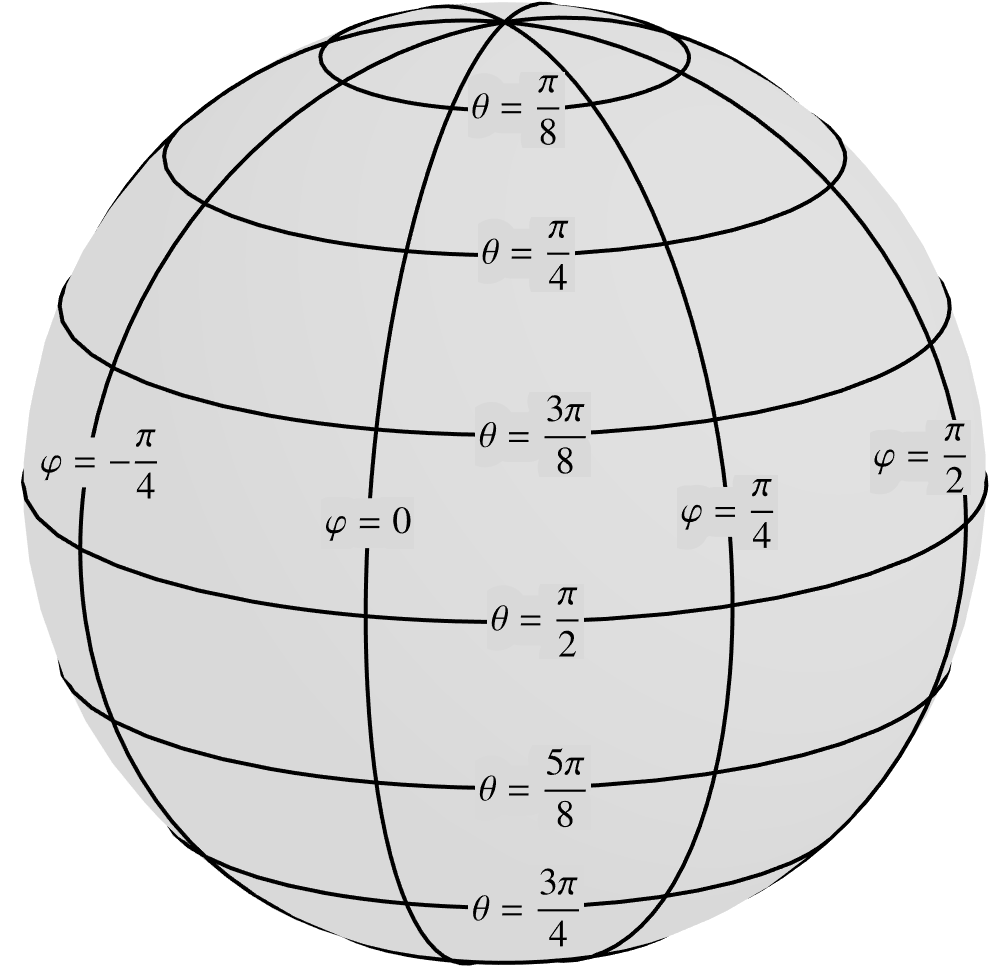 (20.41) the resulting metric tensor
corresponds to
(20.41) the resulting metric tensor
corresponds to
(20.41) which is precisely the metric tensor
in the present example. Therefore, this Riemannian space may be said to be induced from a
surface embedded in a Euclidean space. This example shows that some surfaces embedded in
Euclidean spaces are themselves examples of non-Euclidean spaces. Note that the Gaussian curvature
for embedded surfaces has a beautiful geometric interpretation that will be discussed in a future
book.
20.5The concept of a tensor in Riemannian spaces
Before we can discuss the concept of a tensor, we must first talk about coordinate changes.
Heretofore, our analysis of coordinate changes has been based on the equations of coordinate
transformation
that related two alternative coordinate systems: the "original" unprimed coordinates and
the "new" primed coordinates .
However, it is important to understand the crucial role that the Euclidean space played in
establishing these equations. Given two alternative coordinate systems and
,
consider a specific set of unprimed coordinates, such as . How does one determine the values of the
primed coordinates
that correspond to the above values of the unprimed coordinates? This is done in two steps. The
first step is to identify the physical point in the
Euclidean space corresponding to unprimed coordinates . The second step is to observe the primed
coordinates corresponding to the same point , e.g. . By this mechanism, the function maps to , while maps back to .
With the Euclidean space no longer in the picture, we will take the equation
as the definition, rather
than a description, of the coordinate change. The range of the function defines the domain of the "new" primed
Riemannian space with coordinates .
The inverse mapping function is denoted by , i.e.
Naturally, the definitions of the
Jacobians and
remain the same as before:
The definition of a tensor under such changes of coordinates will remain the same as before, i.e.
is a
tensor with a representative collection of indices if and
are
related by the identity
However, the application of this
condition to some objects is not the same as before as the following example will illustrate.
Consider a Cartesian Riemannian space, i.e. with
the metric tensor field that
corresponds to the matrix
Consider the following equations of
coordinate transformation
Of course, we recognize these equations as a transformation from Cartesian coordinates to
cylindrical. For example, the point maps to the point . Thus, the primed Riemannian space is associated
with the domain . The inverse equations of coordinate
transformation are, of course,
The primed Riemannian space is not yet complete since we have not specified the metric tensor field
. Since our goal is to preserve
the tensor framework, cannot be assigned arbitrarily,
nor can it be assigned by mapping the unprimed metric tensor to
the primed space (which, in this example, would mean that also
corresponds to the identity matrix).
The only logical thing to do is to construct the metric tensor in
the primed coordinate space according to the equation
Notice that this equation was not
given the number (13.59) of the same equation in Chapter 13 to highlight the fact that it now serves as a definition rather
than a corollary. Also note that in this approach, the coordinates are
truly primary while all other coordinate systems are secondary. This loss of parity among
coordinate systems is caused by the absence of an independent Euclidean space acting as an a
priori absolute reference.
To calculate the elements of ,
note that
Therefore,
corresponds to matrix product
which evaluates to the familiar
matrix
In summary, we define the metric tensor so
as to make
transform according to the tensor rule. Similarly, we will augment the notion of a vector by
stipulating that it transforms according to the tensor rule
In other words, a Riemannian
vector is, by definition, a first-order tensor. In general, for every object defined
arbitrarily in the unprimed Riemannian space, we must specify the precise rule by which the object
transforms under a change of coordinates to the primed space.
For all other objects, the question of transformation under a change of coordinates can be
subjected to the same analysis as before and will reach the same conclusions. This applies to such
objects as the contravariant metric tensor ,
the volume element , the
Christoffel symbol , the
Riemann-Christoffel tensor , and
the Levi-Civita symbols and
.
Once the metric tensor is
constructed in the primed Riemannian space, the objects , ,
,
, and
can be constructed from it. Thus, we can study the rules by which they transform between the two
spaces and, because they have the same definitions as they did in Euclidean coordinate spaces, we
will, of course, discover that they transform by the exact same rules.
Finally, it must be noted that the concept of a tensor is stronger and more absolute in a Euclidean
space than in a Riemannian space. In a Euclidean space, an invariant constructed from tensors
represents an object with a clear geometric meaning. Thus, the tensor framework connects the
coordinate space to an independent physical reality which serves as a guarantor of the framework's
meaningfulness. In a Riemannian space, there is no such independent physical reality that can be
used as an absolute reference. Thus, the tensor framework serves as a tool for transferring the
principles developed in Euclidean spaces to a new algebraic setting. It brings with it a certain
degree in internal consistency. For example, the tensor property continues to be reflexive,
symmetric, and transitive as described in Section 14.12.
On balance, however, the tensor framework in the context of a Riemannian space should be seen as a
metaphorical extension of Euclidean ideas.
20.6The arithmetic space
A Riemannian space is, first and foremost, an algebraic structure. In a way, its very purpose is
to provide a framework where analysis can be performed without a need for geometric intuition. It
is somewhat ironic, then, that, being a subset of , a
Riemannian space can be visualized as a Cartesian coordinate grid in a Euclidean space. And not
only that, this geometric view of a Riemannian space is actually beneficial.
For example, consider the Riemannian space induced from a Euclidean plane referred to polar
coordinates .  (20.57) In the spirit of Riemannian spaces, we will refer to the
coordinates as and
instead of and . The induced
Riemannian space occupies the domain . The metric tensor corresponds to the matrix
(20.57) In the spirit of Riemannian spaces, we will refer to the
coordinates as and
instead of and . The induced
Riemannian space occupies the domain . The metric tensor corresponds to the matrix
(20.57)When asked to visualize the domain , all of us, without exception, visualize a
semi-infinite rectangular strip of height . Furthermore, the points
corresponding to integer (or any regularly spaced) values of and
form
a regular grid. The result is nothing but a Euclidean space referred to Cartesian coordinates. We
will refer to this space as the arithmetic space associated with the Riemannian space. Of
course, any Riemannian space, not just induced ones, may be visualized as an arithmetic space.  (20.59) The metric tensor, an essential part
of the Riemannian space, is not reflected in this picture and thus remains behind the scenes.
Surprisingly, the geometry that takes place in the arithmetic space will play an important role in
many of our future analyses. For example, the divergence theorem will be proven by first
demonstrating it in the arithmetic space.
(20.59) The metric tensor, an essential part
of the Riemannian space, is not reflected in this picture and thus remains behind the scenes.
Surprisingly, the geometry that takes place in the arithmetic space will play an important role in
many of our future analyses. For example, the divergence theorem will be proven by first
demonstrating it in the arithmetic space.
(20.59)We must point out the obvious that for induced Riemannian spaces, the arithmetic geometry may look
quite different from the original geometry from which the Riemannian space had arisen. For example,
consider a curve in a Euclidean plane given by the following equations in polar coordinates  (20.62) On the other hand, if we consider the curve in the arithmetic
space given by the same equations, we will observe a straight line:
(20.62) On the other hand, if we consider the curve in the arithmetic
space given by the same equations, we will observe a straight line:  (20.63) Thus, the actual curve and its arithmetic manifestation have
two completely different shapes. In other words, the arithmetic space corresponding to an induced
Riemannian space is a gross distortion of the associated Euclidean space.
(20.63) Thus, the actual curve and its arithmetic manifestation have
two completely different shapes. In other words, the arithmetic space corresponding to an induced
Riemannian space is a gross distortion of the associated Euclidean space.
Of course, we recognize this shape as a spiral
(20.62)(20.63)A more vivid example of the same effect is the familiar distortion that occurs when the spherical
Earth is represented on a flat map. The distortion is especially apparent near the poles where the
volume element is particularly small. 
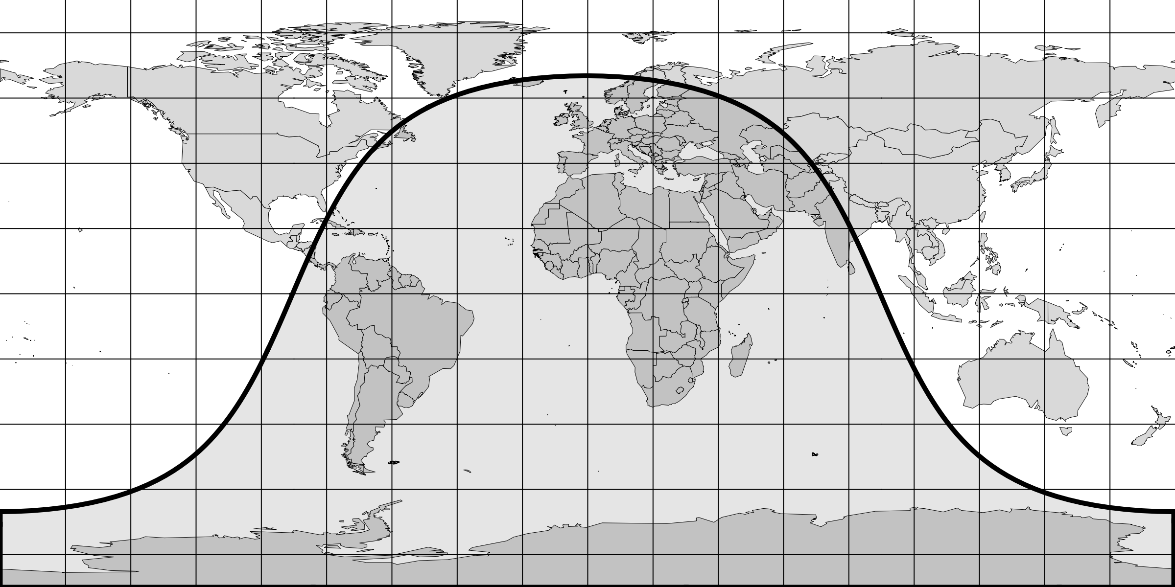 (20.64) The degree to
which the shape of a great circle can change is also a striking illustration of the deformation.
The great circle in the figure above is the terminator, i.e. the line that separates day and
night.
(20.64) The degree to
which the shape of a great circle can change is also a striking illustration of the deformation.
The great circle in the figure above is the terminator, i.e. the line that separates day and
night.
(20.64)Let us be reminded however that, despite the discrepancy between the Euclidean and the
corresponding arithmetic spaces, the availability of the metric tensor
assures that the arithmetic space retains all of the necessary information to perform Euclidean
analysis. For example, suppose that the equation
described the trajectory of a
material particle. Given these equations of motion we cannot easily imagine the actual Euclidean
trajectory of the material particle. Nevertheless, we can calculate the components of its velocity
and acceleration and calculate their magnitudes. Specifically, the components of the velocity are
given by the equation
while the components of the
acceleration are given by
Note that the availability of the
Christoffel symbol is crucial for the latter calculation. With the help of the metric tensor, the
magnitude of the velocity is given by
while that of the acceleration is
given by
We can also calculate the total
distance traveled between the times and
according to the equation
In summary, the fact that the
arithmetic space is severed from the Euclidean space does not in any way preclude us from doing
virtually any kind of analysis short of visualizing the actual shapes.
Finally, going slightly beyond our present scope, note that in terms of the equations of motion
, the components of
acceleration are given by
Thus, if the particle is moving
uniformly in the Euclidean space and therefore its acceleration is zero, then the equations of
motion are characterized by the identity
known as the geodesic
equation. In a Euclidean space, the shortest curve connecting two points is a straight line
and, thus, the geodesic equation tells us whether represents uniform motion along a straight
line.
In a general Riemannian space, the length of a section of a curve given by is defined by the integral
It can be shown that the geodesic
equation represents a form of the Euler-Lagrange equation for the above integral and thus
characterizes the shortest path, again in the Riemannian sense, between two points. The discussion
of the geodesic equation is beyond the scope of this book because it is best discussed in the
context of the Calculus of Moving Surfaces where it can be given a more general treatment.
20.7Arithmetic Euclidean space
At the very outset of our narrative, we defined a Euclidean space as the physical space of our
everyday existence in which the axioms of Euclidean geometry are valid. In particular, we have
relied heavily on two unique characteristics of Euclidean spaces. First, Euclidean spaces can
accommodate straight lines in any direction. This enabled us to introduce, and work freely with,
geometric vectors. Secondly, Euclidean spaces admit Cartesian coordinate systems characterized by
regular orthogonal coordinate grids. As a result, the metric tensor corresponds to the identity
matrix at all points.
Between these two advantages, the former outweighs the latter. The methods of Tensor Calculus
almost completely mitigate the effects of complicated coordinate systems. In fact, this subject's
commitment to avoiding the use of special features of coordinate systems is one of the keys to its
success. On the other hand, the use of geometric vectors was instrumental in stimulating our
geometric intuition and helping us organize information in a very appealing way. Compared to the
collection of coordinates ,
the geometric vector is a
tangible object that connects our analytical investigations to our geometric intuition.
Furthermore, compared to ,
is a
variant of lower order and is therefore simpler. Finally, geometric vectors help guide our
analytical intuition in manipulating coordinate expressions as our mind becomes trained to look for
the geometric-vector interpretation.
Unfortunately, Euclidean spaces, according to our geometric definition, are limited to three or
fewer dimensions. In higher dimensions, the only construct available to us is the Riemannian space.
However, in a Riemannian space, i.e. a subset of
paired with an arbitrary metric tensor field, there is no such thing as a geometric vector. In the
absence of geometric vectors, a first-order tensor
is condemned to variance for a greater part of our analysis. We can determine its invariant dot
product with another vector
as
and its invariant length as the square root of the dot product with itself, but it otherwise
remains in its intermediate variant state devoid of an immediate geometric interpretation.
However, having learned the great utility of boldface symbols in organizing our ideas in the
Euclidean space, we would like to extend it to Riemannian spaces. This can be accomplished by
introducing a construct referred to as the arithmetic Euclidean space in the following way.
An arithmetic Euclidean space is a Riemannian space that occupies the entirety of where
the metric tensor
corresponds to the identity matrix. At all points, the elements of the
covariant basis, denoted by ,
correspond to the
column of the identity matrix. For example, in ,
Then, for a tensor of
order one, the invariant is defined
by
20.7.1The Frenet equations in higher dimensions
As an illustration, we will extend the Frenet formulas to higher dimensions. Recall that the
Frenet equations read
where the subscript denotes differentiation with respect to arc
length .
Part of the what makes the Frenet equations so elegant is the skew-symmetric property of the
matrix. It turns out that this feature persists to higher dimensions.
Consider a curve embedded in an -dimensional arithmetic Euclidean space.
Suppose that the curve is referred to its arc length and is specified by the equations
Let be the
unit tangent to the curve. Then
This definition enables us to avoid
introducing the position vector , which can
certainly be done but is not necessary. Subsequently, however, we will not refer to the components
of or any
of the other vector quantities going forward.
The identity above defines the initial vector from
the local frame. Subsequently, the unit vector is
obtained from by applying the
Gram-Schmidt algorithm in order to make it orthogonal to each of the preceding vectors, and
subsequently factoring out a positive scalar to make it unit length. Finally, the normality of
is
assured in a slightly different way, that you may already anticipate.
Let us investigate the construction of from
. Since , differentiating both sides with respect to yields from which it follows that is orthogonal to . Let
be the
length of and let be the
unit vector that points in the same direction as ,
i.e.
Let us now move on to the next step and analyze
which, by a previously used argument, is orthogonal to , i.e.
Differentiating this identity with
respect to yields
since and
therefore , we
find
Thus, the vector
is orthogonal to both and
and
can therefore be used to define the unit vector and
the corresponding absolute curvature by the
equation
This identity can also be written in
the form
that will serve as the second Frenet
formula.
We now embark on the inductive step of the procedure. The vector is
determined by the condition that it is unit length, i.e.
and is orthogonal to all preceding
vectors , i.e.
Furthermore, we presume that for all
between and , we have the Frenet formulas
Differentiating the orthogonality condition, yields
Substituting the condition
yields
The dot product
vanishes for all by
orthogonality. Meanwhile, the dot product
vanishes for all by orthogonality and equals for . Therefore, the above equation tells us that
and
In other words, is
orthogonal to ,
and, of course, , but
not . The
vector
is, therefore, orthogonal to all
vectors and
can be used to introduce the unit vector and
the absolute curvature :
Rewriting this equation in the form
gives us the
Frenet equation.
We can continue in this fashion until . Following the pattern with the Frenet equations in three
dimensions, the unit vector is
chosen so that the set of vectors is
positively oriented. Then is
chosen so that the identity
is satisfied and, thus, can
be either positive or negative and can rightfully be called the torsion. If the curve is
called right-handed and then it is called
left-handed.
Finally, we note that by the same argument as above, is
orthogonal to all except
and
that
Thus,
is orthogonal to all vectors . Since
our analysis is taking place in dimensions, we conclude that this vector
equals , i.e.
Thus, the
Frenet equation reads
In summary, the Frenet equations
read
20.8Exercises
Exercise 20.1Show that from the intrinsic definition of the Christoffel symbol, i.e.
it follows that
Exercise 20.2Show that the Riemann-Christoffel tensor is skew-symmetric in its last two indices, i.e.
Exercise 20.3Using the formula
present the covariant Riemann-Christoffel tensor
in the form
Exercise 20.4From the form obtained in the previous exercise, show that the Riemann-Christoffel tensor is skew-symmetric in its first two indices, i.e.
and that it is symmetric with respect to switching the first two indices with the last two, i.e.
Exercise 20.5Show that the skew-symmetric property
can also be deduced from
and
Exercise 20.6 Show the first Bianchi identity
Exercise 20.7 Show the second Bianchi identity
Exercise 20.8Show that
and, similarly,
Exercise 20.9Show that the skew-symmetries of the Riemann-Christoffel tensor imply that it vanishes in a one-dimensional space. Alternatively demonstrate this fact by an explicit calculation on the basis of the definition
Exercise 20.10Show that the Ricci curvature tensor defined by the identity
is symmetric, i.e.
Exercise 20.11Show the general commutator formula
A good approach is to consider a first-order variant
and to use the already-established formula for the commutator as the starting point.
Exercise 20.12Show that in a two-dimensional Riemannian space, the Ricci tensor curvature is given by
Therefore, the Gaussian curvature is half the scalar curvature, i.e.
Exercise 20.13In a two-dimensional Riemannian space, suppose that the metric tensor field is diagonal, i.e.
This, for instance, is the case for a Riemannian space induced from a Euclidean plane referred to an orthogonal coordinate system. Show that
In particular, if , then
Exercise 20.14Suppose that the metric tensor that corresponds to the matrix
where is a constant. Show that the nonzero elements of the Christoffel symbol are
Furthermore, the Gaussian curvature is given by
and therefore the Riemann-Christoffel tensor is given by
Exercise 20.15Show that for a metric tensor that corresponds to the matrix
the Gaussian curvature is given by
and, therefore,
Thus, for , for which corresponds to polar coordinates, we have, as expected, . For , on the other hand, the corresponding metric tensor cannot be induced from a Euclidean space.
Exercise 20.16In a three-dimensional space, let
Show that is symmetric, i.e.
Furthermore, can be recovered from by the formula
Problem 20.1Show that, owing to the symmetries present in the Riemann-Christoffel tensor, the number of available degrees of freedom in an -dimensional Riemannian space is