18.1Introductory remarks
Vector Calculus extends the ideas of Calculus to vector fields. As such, one would expect Vector
Calculus to be full of remarkable connections and elegant identities. This is, in fact, so -- but
only when the right language is chosen for the description. Surprisingly, the language of geometric
vectors, which has served us so well in our initial explorations, proves to be ill-equipped at
dealing with even some of the most elementary combinations involving vector fields and their
derivatives..
To illustrate this point, consider the dot product of two vector fields and . Since is a scalar field, it is subject to
the gradient operator . As a
matter of fact, the combination is commonly found in numerous applications.
And since the gradient satisfies the product rule
for scalar fields, we expect to find
a similar rule for the dot product of vector fields, i.e.
However, this identity is
nonsensical as there is no such thing as since the gradient cannot be applied to a vector
field. Thus, we have failed in one of the most elementary endeavors of Vector Calculus.
To understand the root cause of the problem, let us borrow one of our own paragraphs from Chapter
2 in which we addressed the effectiveness of the
language of geometric vectors: As we will quickly discover, working with geometric quantities
leads to greater organization of thought. Geometric vectors have fewer algebraic capabilities
compared to numbers. This is a positive: the small number of accessible operations focuses our
attention on the few that are available. However, when it comes to more sophisticated analyses,
what has been a positive will now become a negative. Geometric vectors are simply not rich enough
algebraically to accommodate the more advanced demands of Vector Calculus.
There are two possible ways out. The first way, and one that is central to our narrative, is to
introduce coordinates in order to switch from vectors to their components. In a
microcosm, the immense utility of this approach can be illustrated by the aforementioned gradient
of a dot product
In terms of components, the dot
product is and
the components of the gradient are given by
Next, an effortless application of the product rule for the covariant derivative yields
Naturally, the gradienttextbf{
} itself is produced by contracting with ,
i.e.
and the calculation is complete.
Note, however, that the restoration of the geometric invariant need not take place at this point if further
analysis is to be conducted. And, although the combinations and
are
devoid of direct geometric interpretation, they can be easily subjected to further analysis.
Meanwhile, the geometric meaningfulness of the eventual results is assured by the tensor framework.
In summary, the identity
has all the simplicity and the structure of its meaningless counterpart
and at the same time enables us to
take full advantage of the tensor framework.
The alternative approach, known as dyadic, doubles down on the geometric aspect of vectors
in order to avoid the use of coordinate systems at all costs. In the dyadic approach, all objects
are assigned some invariant meaning characterized by their interactions with other objects. For
example, the object would be described as a linear
transformation that can be applied to any other vector with the result denoted by , , or simply by . No doubt, this operation would be
defined in such a way that it produces, without mentioning it explicitly, the vector , thus
achieving the same result, but axiomatically and without a reference to the components of vectors.
This simple example illustrates the unfortunate side effect of the dyadic approach: the need for
new kinds of objects and new kinds of operators. The resulting framework never reaches algebraic
closure, i.e. a framework with a finite number of kinds of objects and operators where the result
of applying an existing kind of operator to an existing kind of object always produces an object of
an existing kind. A visit to the Vector calculus identities page on Wikipedia reveals
identities such as
where each identity clearly attempts to capture the elementary product rule, but is only able to do
so by relying on novel kinds of objects and operators. This experience is perfectly captured by
Hermann Weyl's quote from his classic Space Time Matter: In trying to avoid continual
reference to the components we are obliged to adopt an endless profusion of names and symbols, in
addition to an intricate set of rules for carrying out calculations, so that the balance of
advantage is considerably on the negative side. An emphatic protest must be entered against these
orgies of formalism which are threatening the peace of even the technical scientist.
Let us, then, set the dyadic approach aside and concentrate on the coordinate approach supported by
the techniques of Tensor Calculus. In this Chapter, we will discuss four classical differential
operators: the gradient, the divergence, the Laplacian, and the curl. Of course, each one of these
operators is some combination involving the covariant derivative. This highlights one of the
strengths of Tensor Calculus: its highly restricted set of underlying operations. In a Euclidean
space, all objects and operations are expressed in terms of addition, multiplication, contraction,
and the higher-level construct of the covariant derivative.
When a coordinate system is
imposed upon a Euclidean space, we are automatically provided with a number of tensors that can be
used in various combinations, including the covariant and the contravariant bases and
, the
metric tensors and
,
and the Levi-Civita symbols and
.
These basic elements, along with the covariant derivative will
act as jigsaw puzzle pieces in the construction of the invariant differential operators.
Interestingly, the metric tensor will rarely appear explicitly in our expressions since, thanks to
index juggling, it gets absorbed into the tensor with which it is contracted. Nevertheless, its
continual presence is revealed in the placement of indices.
18.2The gradient, the Laplacian, and the divergence
18.2.1The gradient
For a scalar field , one way to
form a differential invariant is to contract with ,
resulting in the vector
We instantly recognize this
combination as the gradient of , which can
also denoted by the symbol , i.e.
Note that a similar combination cannot be formed for a vector field since the
product is
meaningless. This reminds of the fact that we mentioned in Chapter 4 that there is no such thing as the gradient of a vector field. That said,
the dot product and
, which is discussed below, is quite meaningful.
18.2.2The Laplacian
Another meaningful invariant combination involving a scalar field is . This operation is known
as the Laplacian of and can be
denoted by , i.e.
Unlike the gradient, the Laplacian
can be applied to vector fields. Indeed, the combination
represents is a perfectly
well-defined tensor expression. For instance, the Laplacian can be applied to the position vector
and it is
left as an exercise to show that the result is zero. Since the Laplacian of an invariant is itself
an invariant, it immediately raises the question of its geometric interpretation. While some
invariants do not have a simple geometric interpretation, the Laplacian does, and it will be
described later in this Chapter.
18.2.3The divergence
Among combinations that can be applied to first-order tensors , the
most natural one is, undoubtedly,
known as the divergence of
the tensor field . Note
that the Laplacian of a scalar (unrelated to
in
the previous sentence) is equivalent to the divergence of the tensor .
The divergence can
also be thought of as being associated with the vector field . Thus,
the combination can
be referred to as the divergence of the vector field and, in
that context, be denoted by or , i.e.
textbf{ }It is left as a simple
exercise to that is
given by the equation
18.2.4A note on the instructive utility of Tensor Calculus
The logic that has led us to the gradient, the Laplacian, and the divergence illustrates that the
tensor framework not only provides us with a framework for analyzing the invariant properties of a
given object, but also gives us clear and exhaustive instructions for constructing new invariants.
For example, observe that an invariant combination must have an even number of indices and,
therefore, is the least nonzero number of indices that an invariant
can have. Thus, from this "orchestration" point of view, it is a trivial observation -- and yet it
is a profound insight -- that the gradient, the Laplacian, and the divergence are the only possible
invariant expressions involving the symbols , , , , and
--
with the implied possibility of index juggling. Of course, since the Laplacian is the divergence of
gradient, we could reduce the number of elementary differential operators to two, but it is
worthwhile to treat the Laplacian as an equal partner.
More complicated invariant expressions with an even number of indices, such as ,
, and ,
can always be viewed as combinations of the gradient, the Laplacian, and the divergence. For
example, the combination
is the Laplacian of the gradient of , which
becomes apparent when the expression is rewritten as
with parentheses added strictly for
stylistic purposes. Meanwhile, is the Laplacian of the
Laplacian of . This
combination is known as the biharmonic operator and plays an important role in the theory
elasticity. Finally,
when rewritten as
is easily identified as the
Laplacian of the divergence of .
Of course, with the introduction of additional objects, further invariant operators can be formed.
For example, with the help of the Levi-Civita symbol
in two dimensions, we can form the combination
which is the two-dimensional version of the classical curl. In three dimensions, the
combination
leaves a free index that can be contracted with to
form the combination , which
is the actual curl. We will discuss the curl, both in two and three dimensions, later in the
Chapter. Meanwhile, we will turn our attention to the geometric interpretations the Laplacian and
divergence, having described the geometric interpretation of the gradient in Chapter 4.
18.3The geometric interpretation of Laplacian
Suppose that a scalar field describes an
equilibrium temperature distribution in a room. Such a distribution is typically not uniform: it
may be colder near a window and warmer near a radiator. Empirically, we know of this distribution
that there cannot be a point inside the room that is, say, hotter than all of its immediate
neighbors. If such a distribution were to occur in the absence of heat sources -- for example, a
moment after a candle is extinguished -- the temperature would begin to average out until an
equilibrium as achieved where, once again, no point is hotter than its neighbors. Thus, we may
decide to model an equilibrium distribution as one where the temperature at each point is exactly
the average of its neighbors in some precise mathematical sense. That precise sense can be provided
by the Laplacian. In this Section, we will show that the Laplacian of captures
the deviation between the value of at a point
and the average of its values on a small sphere centered at that point. Thanks to this
property, an equilibrium temperature distribution may be characterized by zero Laplacian, i.e.
Functions whose Laplacian vanishes
are known as harmonic and occupy an important place in applied mathematics. If a temperature
distribution is not equilibrium, then its return to equilibrium is naturally modeled by the heat
equation
which essentially states the rate of
change in temperature at a given point is proportional to its deviation from the average of its
neighbors. This canonical example shows how this interpretation of the Laplacian leads to numerous
physical applications.
Let us now derive the precise way in which the Laplacian captures the deviation between the value
of at a point
and the average of its values on a small sphere centered at that point. Consider a scalar field
in a
neighborhood of a point in a
two-dimensional Euclidean space, i.e. a plane, where a sphere is replaced by a circle. Refer the
plane to Cartesian coordinates with the point at the
origin. Recall that in Cartesian coordinates, the Laplacian is given by the equation
In the vicinity of , we can
approximate the function by the first two terms of its Taylor series,
i.e.
where all of the derivatives are evaluated at .
Next, consider a circle of radius centered at
. 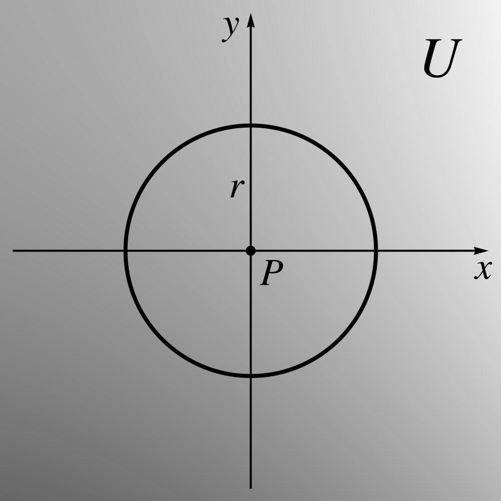 (18.22) If the circle is parameterized by the
equations
(18.22) If the circle is parameterized by the
equations
(18.22)
then the average of the values of over the
circle is given by the integral
Substituting the Taylor series
approximation for and
evaluating the resulting integral, we find
where we see the expression of the
Laplacian emerging on the right. Indeed, the leading term in the difference between and is directly proportional to the
Laplacian, i.e.
This equation captures the precise
sense in which the Laplacian is a measure of the deviation between the value of a function and the
average of its neighbors.
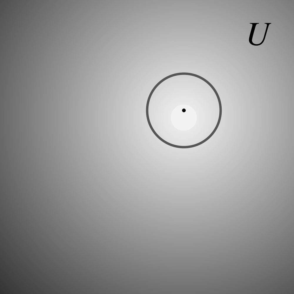
In the following figure, the function illustrated by the contour plot on the left is characterized
by a small value of the Laplacian. By contrast, the function on the right has a high value of the
Laplacian. 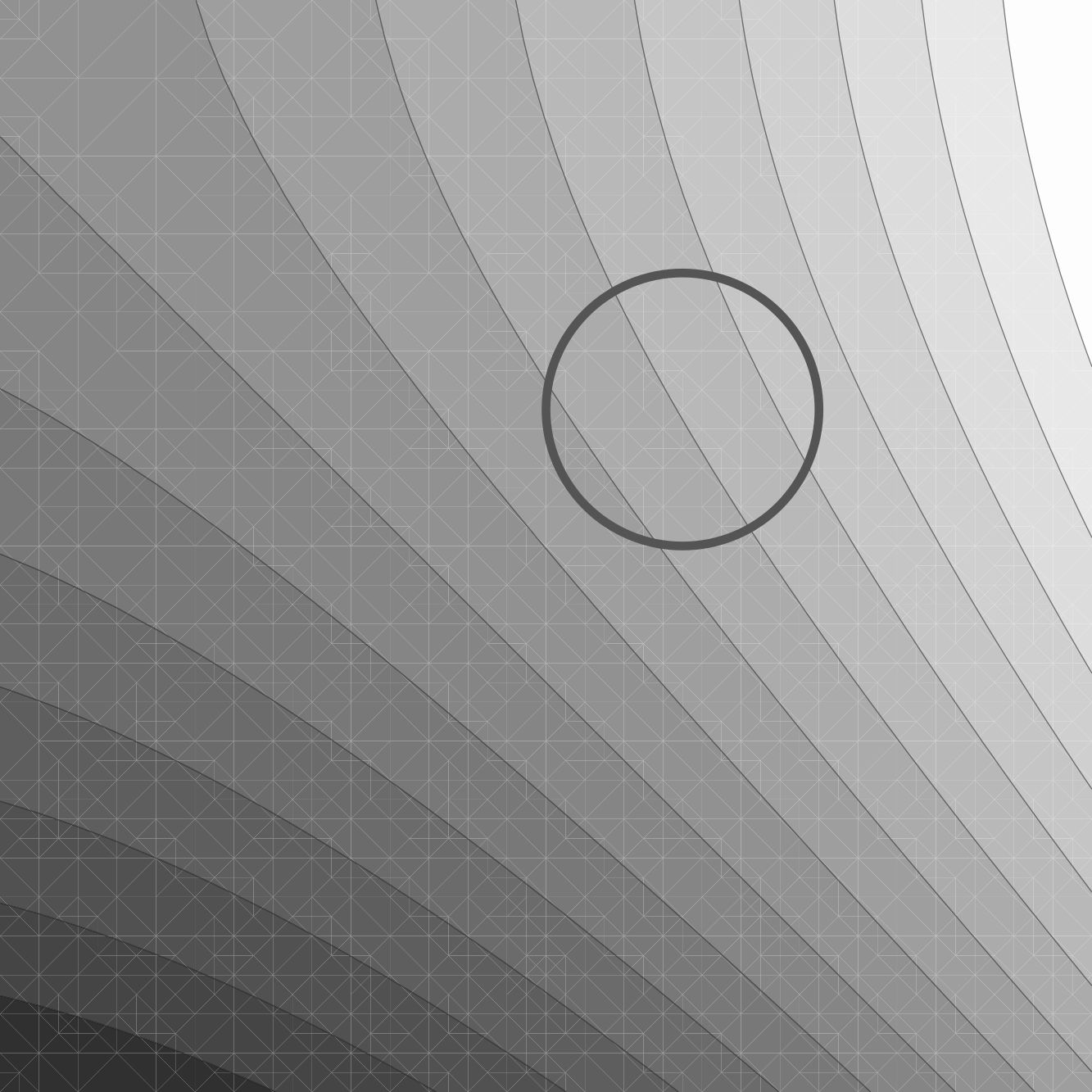
 (18.28)
(18.28)18.4The geometric interpretation of divergence
The geometric interpretation of divergence comes from the divergence theorem, a crucial
generalization of the Fundamental Theorem of Calculus from one-dimensional intervals to
higher-dimensional domains. The divergence theorem and its applications represent a vast topic that
we will discuss in a future book. For the sake of the present discussion, however, we will give the
statement of the theorem here.
Consider a closed domain with boundary and
outward unit normal with
components .  (18.29) For a vector field with
components , the
divergence theorem reads
(18.29) For a vector field with
components , the
divergence theorem reads
(18.29) In dyadic terms, the divergence
theorem appears in the form
The geometric interpretation of the
divergence of which we
are currently pursuing can be gleaned from the integral on the right.
For simplicity, consider a uniform vector field in the
vicinity of a straight boundary characterized
by the normal .  (18.32) This simple configuration will help
us demonstrate that the dot product corresponds
to the flux of across
, i.e. the
rate at which the fluid mass crosses the interface. We will begin by considering the two extreme
examples illustrated in the following figure.
(18.32) This simple configuration will help
us demonstrate that the dot product corresponds
to the flux of across
, i.e. the
rate at which the fluid mass crosses the interface. We will begin by considering the two extreme
examples illustrated in the following figure. 
 (18.33) The left plot shows a flow
parallel to the boundary . In this
case, no fluid crosses and therefore
the flux is zero. Correspondingly, the dot product vanishes
and therefore so does the integral . The right plot shows a
flow orthogonal to the boundary, which results in the greatest flux. Correspondingly, attains its
maximum value, which equals the magnitude of , and the
integral indeed corresponds to the
rate at which the fluid mass crosses the interface , i.e. the
flux.
(18.33) The left plot shows a flow
parallel to the boundary . In this
case, no fluid crosses and therefore
the flux is zero. Correspondingly, the dot product vanishes
and therefore so does the integral . The right plot shows a
flow orthogonal to the boundary, which results in the greatest flux. Correspondingly, attains its
maximum value, which equals the magnitude of , and the
integral indeed corresponds to the
rate at which the fluid mass crosses the interface , i.e. the
flux.
(18.32) (18.33)Finally, consider a flow with an angle of attack that equals with respect to the normal . Identify a
segment along the boundary of length and calculate
the amount of fluid that crosses that segment in a period of time .  (18.34) The fluid that
crosses the segment in that time period is contained in the (gray) parallelogram with sides and , and an angle of . The total amount of fluid contained
in this parallelogram corresponds to its area given by
(18.34) The fluid that
crosses the segment in that time period is contained in the (gray) parallelogram with sides and , and an angle of . The total amount of fluid contained
in this parallelogram corresponds to its area given by
(18.34) Thus, the amount of fluid crossing
the segment per unit time and per unit length along the interface is
Since is precisely , we have
Therefore, the integral
represents the instantaneous amount
per unit time of fluid crossing the boundary, which we understand to be the flux. More
specifically, since is the
outward normal, the integral represents the instantaneous rate of fluid escaping the
domain .
Thanks to the divergence theorem  (18.40)
the volume integral
also represents the
instantaneous rate of fluid escaping the domain . In order to obtain an intuitive understanding of in
the local sense, consider a "small" domain over which the field is
approximately linear and the quantity is
therefore approximately constant. If is
small then, correspondingly, the net flux across the closed boundary is also small. Such a flow may
look like the one in the following plot.
(18.40)If, on the other hand, is
large then we expect a large net flow across the boundary. If , the corresponding
flow may look like the one in the following plot.  (18.41) Of course, this is an exaggerated flow meant to illustrate
the point. Nevertheless, these examples make it apparent where the divergence operator got
its name.
(18.41) Of course, this is an exaggerated flow meant to illustrate
the point. Nevertheless, these examples make it apparent where the divergence operator got
its name.
(18.41)18.5The divergence and the Laplacian in special coordinate systems
In this Section, we will derive the expressions for the divergence and the Laplacian in the most
common special coordinate systems.
18.5.1The divergence
Let us start with the divergence
By definition, the covariant
derivative
is given by
Contracting the indices yields the
expression
that is ready for interpretation in
any coordinate system. For future convenience, let us switch the indices and in the second
term, i.e.
Recall that we have encountered the combination
before in the equation
which was later used to demonstrate
the tensor property of the Levi-Civita symbols. Later in this Chapter, we will also use the above
equation in the derivation of the Voss-Weyl formula which provides an alternative approach to
calculating the divergence in any particular coordinate system.
Let us now begin to interpret the equation
in various coordinate systems. In
affine and, in particular, Cartesian, coordinates , where the Christoffel symbols
vanish, we have
In cylindrical coordinates, recall that the nonzero elements of the Christoffel symbol are
Consequently, the three elements of
the contraction are
Therefore, the expression for the
divergence in terms of the contravariant components reads
Note that the first two terms can be
effectively combined into a single term, i.e.
The Voss-Weyl formula discussed
later in this Chapter will clarify for us why the combination
is a natural one.
It is left as an exercise to show that in polar coordinates in a two-dimensional Euclidean space,
the divergence is given by the equation
Finally, let us turn our attention spherical coordinates. Recall that the nonzero elements of the
Christoffel symbol are
and thus the three elements of are
As a result, in spherical
coordinates, we have
Analogously to the divergence, some
of the terms can be combined, yielding the form
which will, once again, be
elucidated by the Voss-Weyl formula described below.
18.5.2The Laplacian
Since the contravariant derivative is given by
the expression for the Laplacian in
terms of the covariant derivatives alone reads
Expanding the covariant derivatives
in terms of partial derivatives, we find the form
suitable for evaluation in various
coordinate systems.
In Cartesian coordinates , the Christoffel symbol vanishes and
the metric tensors correspond to the identity matrix. Therefore, as we found before, we have
In more general affine coordinates,
the most specific form possible is
where the elements of the
contravariant metric tensor
are constants.
In cylindrical coordinates , recall that
and that the nonzero elements of the Christoffel symbol are
Since
corresponds to a diagonal matrix, the only surviving terms in
must have . Combining
these observations yields
As before, the first two terms can
be combined into one, leading to the final form
In spherical coordinates ,
recall that
which is again diagonal, and that
the nonzero elements of the Christoffel symbols for
which are
Upon substituting these values into the equation
and simplifying, we get
where, combining terms as before, we
arrive at the final form
18.5.3A note on the absolute nature of tensor analysis
In this Section, we are experiencing one important feature of tensor analysis. Namely, tensor
expressions can be used to produce coordinate-dependent expressions directly, i.e. without a
reference to another coordinate system. This feature is best characterized by the adjective
absolute which was used in the original name of our subject, the Absolute Differential
Calculus.
An alternative approach, used in virtually all introductory Calculus textbooks, is to define
objects in the context of a Cartesian coordinate system and then to derive their expressions in
other coordinate systems by a change of variables from the Cartesian coordinates. For example, the
Laplacian would be defined by the expression
in some Cartesian
coordinates. Then it would be demonstrated that this expression yields the same value in
all Cartesian coordinates. Finally, a (laborious and error-prone) change of variables from
Cartesian to spherical coordinates would be used to derive the expression
It is safe to say that, in this
regard, the absolute approach of Tensor Calculus is superior. Furthermore, Tensor Calculus does not
stop there. The Voss-Weyl formula, which we are about to describe, makes the Tensor Calculus
approach even more efficient and robust.
18.6The Voss-Weyl formula
The Voss-Weyl formula, named after Aurel Voss and Hermann Weyl, represents an alternative
approach to calculating the divergence. It reads
where is, of
course, the volume element. The advantage of the Voss-Weyl formula is that provides a way of
calculating the divergence, and therefore the Laplacian, without a reference to the Christoffel
symbol.
To prove the Voss-Weyl formula, recall the formula for the divergence
and the fact that we have
encountered the combination
previously in the formula
for the partial derivative of the
volume element . Solving
for , we
have
Substituting this identity into the
above formula for divergence, we find
Upon factoring out , we find
where we observe, by (a reverse
application of) the product rule, that the quantity in parentheses equals
Thus we arrive at the desired result
A direct application of the Voss-Weyl formula to the Laplacian yields
Since the contravariant derivative
is given by
the final expression for the
Laplacian in terms of partial derivatives reads
The Voss-Weyl formula makes it an even simpler task to derive the expressions for the divergence
and the Laplacian in special coordinate systems. For example, taking the most difficult example of
spherical coordinates ,
recall that
and that
Since the above matrix is diagonal,
the Laplacian is given by a sum of three terms, i.e.
which leads directly to the final
expression
Note that the structure of the
Voss-Weyl shows why combinations such as
represent a natural way of grouping
partial derivatives.
In summary, the Voss-Weyl formula offers an elegant way of evaluating the divergence, and therefore
the Laplacian, with less effort while maintaining greater structure within the expressions.
18.7The curl
We will now add the Levi-Civita symbols to the mix, which will give rise to the curl. Since
the order of a Levi-Civita symbol depends on the dimension of the space, one obtains different
kinds of objects in different dimensions. The classical curl is associated with three
dimensions.
In a three-dimensional Euclidean space, consider a vector field with
components . The
curl of , dyadically
denoted by or , is given
by
The components
of are given by
The invariant nature of the curl
immediately follows from the fact that it is defined in terms of tensors and tensor-preserving
operations. As always, we must note that the Levi-Civita symbol ,
as classically defined, is a tensor only with respect to orientation-preserving coordinate
transformations. Therefore, the curl of , as defined
by the above equations, is also a tensor only with respect to orientation-preserving coordinate
transformations. It could be made a full tensor by introducing the orientation scalar , discussed in Section 17.10.
Interestingly, and perhaps somewhat unexpectedly, the covariant derivative in the
equation
can be replaced with the partial
derivative .
Indeed, recall that the Christoffel symbol is symmetric, i.e.
and therefore
as a double contraction of an
alternating system with a symmetric system. Since
we have
Thus,
as we set out to show.
A great mnemonic device for the curl can be formulated with the help of the determinant. Namely,
the curl is given by the formula
where it is understood that
"multiplying" by the covariant derivative means applying it. Since, as we just discovered, the
covariant derivatives can be replaced with partial derivatives, the above formula can be rewritten
as
We observe, therefore, the curl is
given by the same expression in term of partial derivatives in all coordinate systems, save for the
factor of . Thus,
there is no need for documenting the particular expressions for the curl in specific coordinate
systems.
18.8The geometric interpretation of the curl
The geometric interpretation of the curl is that it is a local measure of swirliness in the
vector field . Much like
with the divergence, this interpretation comes from an integration theorem. Namely, Stokes'
theorem which is a form of the divergence theorem that applies to a curved surface patch immersed in a
vector field . It will be
described, along with the divergence theorem, in a future book, but its statement will be given
here for the purposes of our present discussion. 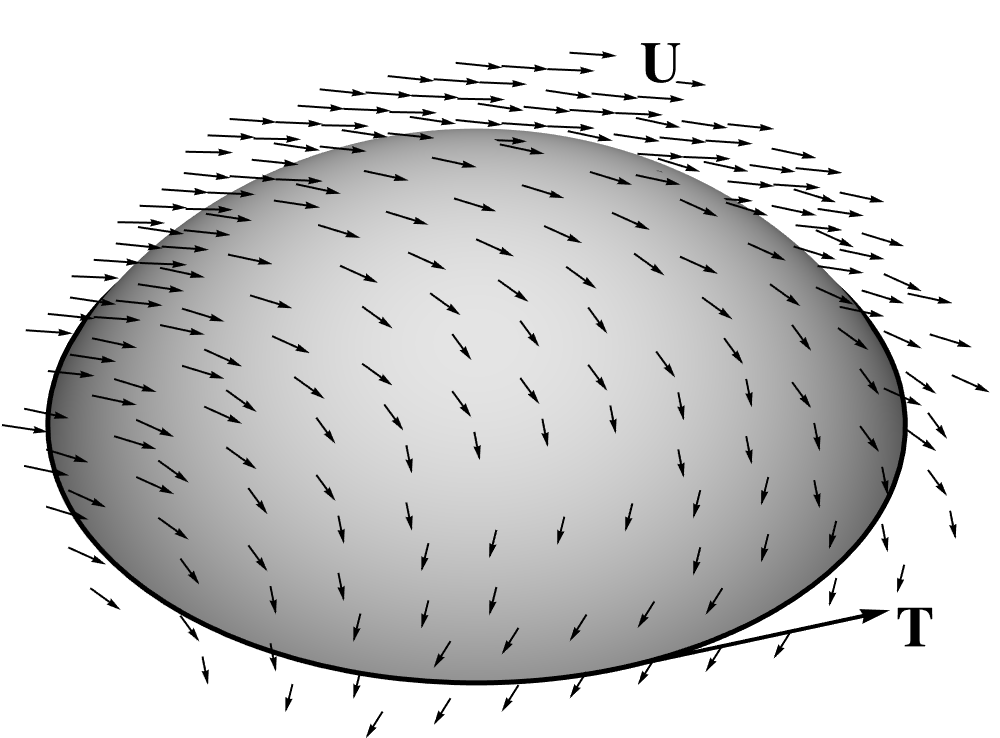 (18.82) If is the unit
normal on a patch and is the unit
tangent along the boundary , then the Stokes' theorem reads
(18.82) If is the unit
normal on a patch and is the unit
tangent along the boundary , then the Stokes' theorem reads
(18.82) As with the divergence, the
interpretation of comes from the contour integral on the right as we consider a
small patch.
In fact, let us consider a small circular patch and note that
the tangent exemplifies
swirliness.  (18.84) At each point on the boundary , the dot product in the
integrand of the contour integral is proportional to the magnitude of and,
importantly, to the cosine of the angle between and , i.e. the
degree to which is aligned
with . Thus, the
contour integral rewards the "likeness" between and and thus
rewards the swirliness in .
(18.84) At each point on the boundary , the dot product in the
integrand of the contour integral is proportional to the magnitude of and,
importantly, to the cosine of the angle between and , i.e. the
degree to which is aligned
with . Thus, the
contour integral rewards the "likeness" between and and thus
rewards the swirliness in .
(18.84)Suppose that the space is referred to Cartesian coordinates so that the circle patch is in the
- and with its center at the origin.
Consider the three different vector fields given by the equations 

 (18.88) It is left as an exercise to show that
and illustrated in the following figure.
(18.88)Due to the swirly character of the vector field in the
first plot, we observe that along the boundary, and are
consistently aligned. As a result, the dot product is positive
everywhere and every point makes a positive contribution to the integral .
Meanwhile, in the other two plots, fails to
exhibit any degree swirliness. In the second plot, is
orthogonal to at each
point resulting in the zero contour integral. In the third plot, varies from
being largely aligned with at some
points to counter-aligned at other points. Consequently, the contributions to the contour integral
from the different sections of the boundary cancel each other, once again resulting in a zero
integral.
As a final remark, note that swirliness may be difficult to judge with the naked eye. For example,
even the swirly field in the first plot does not appear swirly away from the origin.
However, it is equally swirly at all points, as indicated by the constant value of . In order for the swirliness to become visually apparent on a
small patch, one needs to subtract out the average value of the field.
18.9The curl in two dimensions
In a two-dimensional space, the Levi-Civita symbol
has two indices and, thus, there are not enough indices to produce a first-order tensor out of the
combination .
Nevertheless, we can still consider the combination
which produces a scalar invariant , i.e.
As in the case of the
three-dimensional curl, the covariant derivatives can be replaced with partial derivatives and the
result can be captured by the determinant equation
Much like the curl in three dimensions, measures the
degree of swirliness in the field . For the
vector field
which exemplifies swirliness, is given by
18.10Vector calculus identities involving the curl
The identities of Vector Calculus are rarely used in all but the most elementary applications. Most
analyses encounter situations not covered by the common Vector Calculus identities involving , , and the Laplacian. As we already discussed, even
the analysis of a combination as fundamental as requires the introduction of new operators.
Thus, at best, the Vector Calculus identities are incomplete.
In Tensor Calculus, the need for analogous identities simply does not arise. All analyses are built
up from the metrics and the covariant derivative, and proceed according to the limited set of rules
governing the handful of available operations. It is certainly true that any analysis will
reference previously established relationships, such as
However, using such relationships is
simply a matter of convenience since all such relationships can be derived from first principles by
the same limited set of rules. In other words, none of these relationships can be considered
primary in the sense that they must be a priori derived by means outside of the
present framework. Thus, every analysis in Tensor Calculus can, and often does, proceed from first
principles and is guaranteed not to encounter a combination, such as in Vector Calculus, that cannot be reduced to
already-available more primary objects. Ultimately, every analysis in a Euclidean space can be
performed in terms of the covariant derivative and the metrics, which, in turn, can be expressed in
terms of partial derivatives and the position vector. (In a Riemannian space, the covariant metric
tensor replaces the position vector as the primary object and therefore every analysis can be
reduced to partial derivatives and the metric tensor.)
Nevertheless, for illustrative purposes, we would like to use the techniques of Tensor Calculus to
demonstrate some of the most common identities of Vector Calculus, such as
Other identities that may be stated in dyadic terms but whose proof requires coordinate-based
calculations, are left as exercises for the reader.
Let us begin with the first two identities and show that both follow easily from the skew-symmetric
property of the Levi-Civita symbol. Since the components of are , the components of are
varepsilon^{ijk}nabla_{i}nabla_{j}U. Recall that, in a Euclidean space, the covariant derivatives
commute, i.e. nabla_{i}nabla_{j}U=nabla_{j}nabla_{i}U. Consequently, the preceding expression
represents a double contraction between a skew-symmetric system, ,
and a symmetric system, , and therefore vanishes,
as we set out to show.
Turning our attention now to , the components of are and
therefore is given by the expression
By the metrinilic property, the
Levi-Civita symbol "passes through" the covariant derivative, i.e.
and we once again have a double
contraction (on and ) between a
skew-symmetric system, ,
and a symmetric system, .
Therefore, the result is zero as we set out to show.
Finally, let us consider , which will lead to a more intricate analysis.
Let
The components
of are given by
Thus, the components of
are given by
Once again, the Levi-Civita symbol
"passes through" the covariant derivative ,
i.e.
The combination
is given by
as it is left as an exercise to
show. Therefore,
Upon applying the distributive law
and absorbing the Kronecker symbols, we find
Finally, switching the order of the
covariant derivatives in each term (for largely aesthetic reasons), we arrive at the final
expression
Expressed in dyadic terms, the above
identity reads
as we set out to show.
18.11Exercises
Exercise 18.1Show that for a vector field and a scalar field , the divergence satisfies the product rule
Exercise 18.2If and are scalar fields and is a function of two variables, show that
Exercise 18.3By referring to the Christoffel symbol, show that in polar coordinates in a two-dimensional Euclidean space, the divergence is given by
Exercise 18.4Show that the Laplacian of the position vector vanishes, i.e.
Exercise 18.5Use the above formula to show that
where is the dimension of the Euclidean space. For an alternative derivation of this formula, see Exercise 15.5.
Exercise 18.6If is the length of the position vector , show that
where is the dimension of the space.
Exercise 18.7Show that for a constant vector field ,
Exercise 18.8Show that the covariant derivative applied to a cross product of two fields and satisfies the product rule
18.11.1Applications of the Voss-Weyl formula
Exercise 18.9Show that in polar coordinates, where
the expression for the divergence reads
Exercise 18.10Show that the Laplacian of the function
vanishes.
Exercise 18.11Show that in cylindrical coordinates, where
the expression for the divergence reads
Exercise 18.12Show that in spherical coordinates, where
the expression for the divergence reads
Exercise 18.13Show that in cylindrical coordinates, the expression for the Laplacian reads
Exercise 18.14Show that in spherical coordinates, the expression for the Laplacian reads
18.11.2Other exercises{}
Exercise 18.15In three dimensions, show that
where is the position vector. Meanwhile, in two dimensions,
Exercise 18.16Show that for a constant vector field ,
Exercise 18.17Show the identity
from Section 18.10 by justifying each step in the following chain of identities:
Exercise 18.18Show that in a two-dimensional Euclidean space,
In words, the curl of the gradient is zero.
Exercise 18.19Show that the one-dimensional "curl" defined as
corresponds to , i.e. the derivative with respect to the arc-length.
Exercise 18.20Explain why the invariant combination
does not lead to an interesting new differential operator.
Exercise 18.21Decipher and then derive the following identities.