6.1Introductory remarks
A coordinate system is a method for enumerating points in a Euclidean space by numbers. In order
for the coordinate system to be reasonably regular, the number of coordinates must match the
dimension of the Euclidean space, i.e. three coordinates in a three-dimensional space, two
coordinates on a plane, and one coordinate on a straight line. Furthermore, the correspondence
between the points and the coordinates must be reasonably smooth. More precisely, the position
vector should be a
sufficiently differentiable function of the coordinates. Other than this requirement, a coordinate
system may be completely arbitrary.
For a general coordinate system, the coordinates will be denoted by the capital letter with a
superscript, i.e. or,
collectively, . When
indicating the coordinates of a particular point, we will put the coordinates in parenthesis, i.e.
. The unusual placement of the index as a
superscript is a crucial element of the tensor notation which is the bedrock of Tensor Calculus.
Generally speaking, the term tensor notation refers to the use of indices, both as
superscripts and subscripts, to enumerate sets of related objects. Its most basic elements will be
described in Chapter 7. Many of its other important
elements, such as index juggling, will emerge in later chapters.
The use of a superscript for enumerating coordinates is a completely arbitrary choice, and we could
have just as well chosen to use a subscript. However, Tensor Calculus has strict rules for
coordinating the placements of indices. Once we have chosen to use a superscript for coordinates,
the placement of all other indices is uniquely determined.
Obviously, there are an unlimited number of ways to impose a coordinate system upon a Euclidean
space. There are a handful of well-known families of coordinate systems that are frequently used
for analyzing problems with special geometries. The most common coordinate systems in a
three-dimensional space are Cartesian or, more generally, affine coordinates denoted by , cylindrical coordinates denoted by
, and spherical coordinates denoted by
.
In two dimensions, the most common coordinate systems are once again Cartesian or affine
coordinates denoted by and polar coordinates
denoted by .
In two dimensions, a coordinate system can be represented graphically by its coordinate
lines, i.e. curves that consist of points that correspond to a fixed value of one variable
while the other is allowed to vary. The following figure illustrates the coordinate lines for a
generic coordinate system in
the plane.  (6.1) In three dimensions, coordinate lines
are replaced by coordinate surfaces, i.e. surfaces that correspond to a fixed value of one
variable while the other two are allowed to vary. We will use this method of illustrating
coordinate systems for cylindrical and spherical coordinates later in this Chapter.
(6.1) In three dimensions, coordinate lines
are replaced by coordinate surfaces, i.e. surfaces that correspond to a fixed value of one
variable while the other two are allowed to vary. We will use this method of illustrating
coordinate systems for cylindrical and spherical coordinates later in this Chapter.
(6.1)6.2An example illustrating the great utility of coordinates
In the early chapters, we discovered the impressive utility of geometric vectors when treated as
pure geometric objects. However, we also observed the serious limitations of pure geometric
methods. Most of these limitations are removed by the use of coordinate systems. We will now begin
to explore the remarkable power of analytical methods that leverage the utility of coordinate
systems.
For a simple but effective demonstration, let us revisit the problem of differentiating the
vector-valued function that corresponds to the unit circle as changes from to .  (6.2) In Chapter 4,
we solved this problem by a geometric analysis in a coordinate-free setting. Our solution was
intuitive, insightful, and intellectually satisfying. On the other hand, our argument was lengthy
and is, in practice, applicable only to very simple problems. Just imagine an that traces out an ellipse instead of a
circle -- the problem instantly becomes worthy of an eighteenth-century graduate thesis. With the
help of coordinates, the circle and the ellipse are equally simple and the solution is quicker,
more straightforward and more powerful compared to the coordinate-free approach.
(6.2) In Chapter 4,
we solved this problem by a geometric analysis in a coordinate-free setting. Our solution was
intuitive, insightful, and intellectually satisfying. On the other hand, our argument was lengthy
and is, in practice, applicable only to very simple problems. Just imagine an that traces out an ellipse instead of a
circle -- the problem instantly becomes worthy of an eighteenth-century graduate thesis. With the
help of coordinates, the circle and the ellipse are equally simple and the solution is quicker,
more straightforward and more powerful compared to the coordinate-free approach.
(6.2)Introduce a Cartesian coordinate system with the origin at the
center of the circle. Let the unit vectors pointing in the direction of the coordinate axes be
denoted by and .  (6.3) Then is given by the equation
  (6.6) It is clear that the vector is a unit vector orthogonal to . This can also be verified by evaluating the
dot products and . Note that the inner product matrix with
respect to the basis is the identity matrix, i.e.
(6.6) It is clear that the vector is a unit vector orthogonal to . This can also be verified by evaluating the
dot products and . Note that the inner product matrix with
respect to the basis is the identity matrix, i.e.
(6.3) for which differentiation with
respect to readily yields
The resulting analytical expression
for can now be interpreted geometrically. The
following figure shows placed at the tip of .
(6.6) and, therefore, according to the
formula for evaluating dot products in the component space derived in Section 2.6,
and
where the first identity confirms
that is unit length and the second confirms that
it is orthogonal to .
6.3An example illustrating the peril of coordinates
Consider the problem that appeared in Exercise 4.16 in Chapter 4. Given a point and a curve , show that for the point on that is closest to , the segment is orthogonal to .  (6.10) The intended solution was as follows. Let be the vector equation of the curve , where the origin for the position vector is placed
at . The problem then is to find the value of
that yields the shortest vector .
(6.10) The intended solution was as follows. Let be the vector equation of the curve , where the origin for the position vector is placed
at . The problem then is to find the value of
that yields the shortest vector .  (6.11) Denote the objective function by , i.e.
(6.10)(6.11) where we neglected to take the
square root of the right side since for a positive quantity, there is no difference between
minimizing it or its square. Suppose that the minimum of occurs at , i.e.
By the dot product rule
we find that the derivative of is given by
Equating to zero, we conclude that the critical value
is
characterized by the equation
In other words, , which corresponds to the
segment , is orthogonal to the tangent , as we set out to prove.
The great advantage of this approach is, of course, its geometric insight. By considering vectors
themselves rather than their components, we never let go of the geometric meaning and, as a result,
the final identity yielded itself to an immediate geometric interpretation. On the other hand, the
great shortcoming of this approach is that, while it perfectly characterizes the solution in
geometric terms, it does not provide a means of finding it for a specific geometric configuration,
i.e. finding the specific point on a specific
curve that is closest to a specific point .
Let us demonstrate the coordinate approach by attempting the same problem with the help of
Cartesian coordinates. Suppose that the coordinates of the point are and that the curve is given by the functions and .  (6.17) Then the objective function is given by the equation
(6.17) Its derivative is
Equating to , we obtain the desired algebraic equation for , i.e.
The great advantage of this approach is, of course, the fact that, for a specific problem, it can
identify the specific point of the curve that is closest to the point . For example, if is the parabola given by the equations  (6.23) then the equation for reads
and the coordinates of are ,
(6.23) or
An approximate solution of this
equation, , gives a precise location of the
sought after point .
What, then, is the great disadvantage of this approach? It is this: neither the precise numerical
answer for the specific problem, nor the more general equation
yield the geometric insight that
must be orthogonal to the curve.
While it is true that an experienced eye may spot the dot-product structure in the equation above,
keep in mind that this is one of the simplest problems one may encounter. In a more complicated
situation, the geometric interpretation is likely to be irrevocably lost with the introduction of
coordinates. This phenomenon is exemplified by Euler's minimal surface equation
briefly discussed in Chapter 1, which did not yield the geometric insight that a
minimal surface is characterized by zero mean curvature.
The last two examples have demonstrated both the great utility and the great peril of coordinate
systems. The beauty of Tensor Calculus is in its remarkable ability to combine the geometric and
the coordinate approaches in a way that extracts the full benefits of both.
6.4A common ill-advised way of introducing special coordinate systems
In all likelihood, you are already familiar with the most common special coordinate systems
described below. Nevertheless, I hope that you do not skip this discussion since it describes
coordinates systems differently from most textbooks. The common approach of introducing a special
coordinates is by relating it to an a priori Cartesian coordinate system. This approach is
typified by the following figure from the Wikipedia article on spherical coordinates, where one
notices the ever-present background Cartesian grid.  (6.26) Subsequently, spherical coordinates
are related to Cartesian coordinates by the equations
(6.26) Subsequently, spherical coordinates
are related to Cartesian coordinates by the equations
(6.26)
as well as the (more elegant) inverse equations
This common approach violates the spirit of Tensor Calculus by arbitrarily singling out a single
coordinate system -- in this case, the Cartesian coordinates . From the point of view of the
geometric space, this approach is not only aesthetically and philosophically objectionable but is,
in fact, logically flawed since it does not describe how the coordinates were introduced in the first place.
As a result, the construction is, at its very outset, detached from the very Euclidean space that
it is meant to describe. For example, one is not able to answer the question what is the
distance between the points with Cartesian coordinates and ? If one answers , then it would
seem that the presence of the coordinate system has imposed the concept of length upon the parent
Euclidean space. This is contrary to our approach in which the relationship is logically reversed:
the concept of length comes first as an inalienable characteristic of the Euclidean space. Thus,
the better alternative, and one that is consistent with the spirit of Tensor Calculus, is to
describe the coordinate system in absolute terms by referring to the inherent geometric
characteristics of the Euclidean space. This will be our approach.
6.5Cartesian coordinates
Let us start with Cartesian coordinates. Cartesian coordinates are, without a doubt, the
most commonly used -- and misused -- coordinate systems. That said, they are indeed a
natural choice in many situations and, in a number of ways, represent the most easy to use
coordinates. Our initial discussion will focus on the two-dimensional plane, as it is easier to
visualize than the three-dimensional space, but is still sufficiently rich to illustrate all of its
most important characteristics.
Cartesian coordinates are easiest to describe in terms of the coordinate basis . Choose an arbitrary origin and a pair of
unit orthogonal vectors and . To reiterate, in order for the coordinate system to qualify
as Cartesian, the vectors and must be a) orthogonal and b) of unit length. If one of the
conditions is violated, the resulting coordinates are no longer Cartesian, but merely
affine.  (6.33) Given the origin and the pair
of unit orthogonal vectors and , the Cartesian coordinates of a point are the
components of the vector from to with respect
to and , i.e.
(6.33) Given the origin and the pair
of unit orthogonal vectors and , the Cartesian coordinates of a point are the
components of the vector from to with respect
to and , i.e.  (6.35) The resulting coordinate lines corresponding to integer values
of and form a regular square grid spaced by
precisely one Euclidean unit.
(6.35) The resulting coordinate lines corresponding to integer values
of and form a regular square grid spaced by
precisely one Euclidean unit.  (6.36)
(6.33) The corresponding geometric
construction is illustrated in the following figure.
(6.35)(6.36)Another common way of representing Cartesian coordinates is by drawing the coordinate axes.
The -axis is a straight line that passes through
the origin in the
direction of the basis vector . In other
words, the -axis is the coordinate line that corresponds
to . Similarly, the
-axis is a straight line that passes
through in the
direction of the basis vector , and is the coordinate line that corresponds to .  (6.37) This representation is attractive since it is more
uncluttered. For the rest of this Section, however, we will stick with the coordinate line
representation for the sake of consistency with other special coordinate systems.
(6.37) This representation is attractive since it is more
uncluttered. For the rest of this Section, however, we will stick with the coordinate line
representation for the sake of consistency with other special coordinate systems.
(6.37)There are infinitely many Cartesian coordinate systems in the plane since we are free to choose any
point for the origin and any
orientation (in the sense of rotation) of the orthonormal basis vectors and . The following figure illustrates a different Cartesian
coordinate system that differs from the one above in both the location of the origin and the
orientation of and .  (6.38)
(6.38)Finally, we also have the choice of orientation (in the sense of Section 3.1) of the basis . If the vectors and form a positively oriented set, then the coordinate system is
said to be positively oriented or right-handed. Otherwise, it is negatively
oriented or left-handed. The following figure shows a left-handed Cartesian coordinate
system.  (6.39)
(6.39)As we have already mentioned, the requirement that and are unit vectors is essential to the definition of
Cartesian coordinates. Even if and are orthogonal and have equal but non-unit
lengths, the resulting system can no longer be considered Cartesian. For example, the
coordinate system illustrated in the following figure (where the reference segment on the bottom
right has unit length) is not Cartesian, even though its coordinate lines form a regular square
grid.  (6.40) Note that without the reference
segment, there would have been no way of determining whether the system is Cartesian.
(6.40) Note that without the reference
segment, there would have been no way of determining whether the system is Cartesian.
(6.40)In three dimensions, a Cartesian coordinate system is constructed by selecting an arbitrary origin
and a set of
three pairwise-orthogonal unit vectors , , and .  (6.41) Echoing the two-dimensional case, the Cartesian coordinates
of a point are the
components of the vector from to with respect
to , , and , i.e.
(6.41) Echoing the two-dimensional case, the Cartesian coordinates
of a point are the
components of the vector from to with respect
to , , and , i.e.  (6.43) The coordinate system is right-handed or positively
oriented if the set is
positively oriented. Otherwise, it is left-handed or negatively oriented.
(6.43) The coordinate system is right-handed or positively
oriented if the set is
positively oriented. Otherwise, it is left-handed or negatively oriented.
(6.41) The resulting coordinate lines
corresponding to integer values form a regular square grid spaced by precisely one Cartesian unit.
(6.43)6.6Affine coordinates
Affine or rectilinear coordinates are a generalization of Cartesian coordinates
without the constraints of orthogonality and unit length. Affine coordinates are constructed in the
exact same way as Cartesian coordinates from an arbitrary linearly independent set of vectors , , and .  (6.44) Once again, the affine coordinates of a point are the
components of the vector from to with respect
to the vectors , , and , i.e.
(6.44) Once again, the affine coordinates of a point are the
components of the vector from to with respect
to the vectors , , and , i.e.  (6.46) The term rectilinear refers to
the straightness of the coordinate lines. Non-affine coordinate systems are known as
curvilinear.
(6.46) The term rectilinear refers to
the straightness of the coordinate lines. Non-affine coordinate systems are known as
curvilinear.
(6.44) The resulting coordinate lines
corresponding to integer values form a skewed regular parallelepiped grid, as illustrated in the
following figure.
(6.46)The concept of orientation applies to affine coordinates just as well as Cartesian. An affine
coordinate system is said to be positively oriented or right-handed if the set of
vectors is
positively oriented. Otherwise, it is negatively oriented or left-handed.
Any two affine coordinate systems are related by a combination of a linear transformation and a
shift. Suppose that and are
two sets of affine coordinates corresponding to the respective origins at and and
the coordinate bases and . Then
the coordinates and are
related by
where are
the coordinates of in the primed
coordinate system and (the transpose of) the matrix relates the unprimed and primed
coordinate bases according to the formal identity
We can eschew the unwelcome
transpose by organizing the elements of the coordinate bases in rows instead of columns, i.e.
The proof of this property of affine
coordinates is left as an exercise.
Interestingly, the matrix participates in the translation from
unprimed to primed coordinates and -- note the reverse direction -- from primed to
unprimed coordinate bases. Thus, coordinates themselves and their associated bases transform in
fundamentally opposite ways. This simple observation, it turns out, will prove to be the
cornerstone of the tensor framework.
6.7Polar coordinates
Polar coordinates are well suited for a wide range of
geometries in the plane, especially those that are naturally described in terms of the distance to
a reference point, such as the star-shaped region in the figure below. A star-shaped region
is one for which there exists a fixed point from which all points on the boundary are in a direct
line of sight. This allows for a unique mapping between the distance from the fixed point and the
direction. Such shapes can be captured in polar coordinates by a single function.  (6.50)
(6.50)The construction of a polar coordinate system is illustrated in the figure below. Designate an
arbitrary point as the
pole or the origin, and select an arbitrary ray , known as the
polar axis, emanating from . The polar
coordinates of a point are the
numbers and , where is the
Euclidean distance from to the pole and is the
signed angle, measured in radians, between the segment and the
polar axis in the
counterclockwise direction.  (6.51) In order to uniquely determine the numerical value of
the angle , it must be
constrained to a semi-open range of length , such as or . Choosing , for example, results in the coordinate lines
illustrated in the following figure.
(6.51) In order to uniquely determine the numerical value of
the angle , it must be
constrained to a semi-open range of length , such as or . Choosing , for example, results in the coordinate lines
illustrated in the following figure.  (6.52) This figure could be made to appear even more regular by
choosing radial coordinate lines corresponding to multiples of, say, instead
of integer values.
(6.52) This figure could be made to appear even more regular by
choosing radial coordinate lines corresponding to multiples of, say, instead
of integer values.  (6.53)
(6.51)(6.52)(6.53)In some applications, such as analysis of curves, it is often more convenient not to
restrict the range of and to allow
it to be any real number. For example, the following figure shows the curve corresponding to
the equations  (6.56) Consider the point on the curve
in the figure above. Had we not already known the equation of the curve, we may think that the
-coordinate of
is . However,
corresponds
to and, therefore, to . Thus, the choice to allow to take on
arbitrary values results in a great deal of convenience at the cost of uniqueness.
(6.56) Consider the point on the curve
in the figure above. Had we not already known the equation of the curve, we may think that the
-coordinate of
is . However,
corresponds
to and, therefore, to . Thus, the choice to allow to take on
arbitrary values results in a great deal of convenience at the cost of uniqueness.
for the parameter -- and therefore -- ranging
from to .
(6.56)Furthermore, we can also allow the variable to take on
negative values. By convention, the point with
coordinates , where is negative,
is found at the point with proper polar coordinates . In other words, for negative , we find
by moving in
the "negative" direction along the ray corresponding to the angle . A curve
given by the equations  (6.59) Note that the variable changes sign
at multiples of . For a
continuous curve, this change of sign in can occur
only when the curve passes through the origin.
(6.59) Note that the variable changes sign
at multiples of . For a
continuous curve, this change of sign in can occur
only when the curve passes through the origin.
where and therefore assumes
negative values, is shown in the following figure.
(6.59)6.8Cylindrical coordinates
Cylindrical coordinates extend polar coordinates to three dimensions. In order to construct
a cylindrical coordinate system, first, select a plane known as the coordinate plane. The
coordinate plane divides the space into two half-spaces. Arbitrarily select one of the half-spaces
as positive and the other as negative. Construct a polar coordinate system within the
coordinate plane by selecting an arbitrary pole and an
arbitrary ray . The polar
angle increases in
the direction that appears counterclockwise from the positive half-space. Then, to
each point in the space,
assign the coordinates , , and , where and are the polar
coordinates of the orthogonal projection of onto the
coordinate plane and is the
signed Euclidean distance between and the
coordinate plane, i.e. is positive
if is found in
the positive half-space and negative otherwise.  (6.60)
(6.60) The cylindrical or longitudinal axis is the straight line orthogonal to the
coordinate plane that passes through the origin . It consists
of the points for which . The distance
between a point and the
cylindrical axis equals . The term
cylindrical comes from the fact that points characterized by constant form a
cylinder. The other two families of coordinate surfaces are planes.
A selection of coordinate lines for cylindrical coordinates is shown in the following figure.  (6.61) A selection of coordinate surfaces is shown in the following
figure.
(6.61) A selection of coordinate surfaces is shown in the following
figure.
(6.61)6.9Spherical coordinates
Spherical coordinates, denoted by the letters , , and , are perfectly intuitive. Using a planetary analogy, the
angles and correspond to colatitude and longitude on the surface of
the Earth, while corresponds
to the Euclidean distance to the center of the Earth. To construct a spherical coordinate system,
start by selecting an arbitrary origin . The
coordinate of the point
is the
distance between and . Next, select
an arbitrary coordinate plane that passes through . We will
refer to the straight line orthogonal to the coordinate plane that passes through the origin as the
spherical axis. The angle , known as the
colatitude, varies from to and gives the
angle between the segment and the
spherical axis. The remaining coordinate is the azimuth which varies from to . It corresponds to the angle between
the projection of onto the
coordinate plane and a fixed arbitrarily polar axis that passes
through the origin in the
coordinate plane.  (6.63)
(6.63)The points corresponding to a given value of form a
coordinate sphere. If is fixed in addition to , the result
is a "meridian" on the corresponding coordinate sphere. If is fixed in
addition to , the result
is a "parallel". Neither angle is defined at the origin . The azimuth
is undefined along the entire spherical axis. The
following figure shows one coordinate surface for each variable. 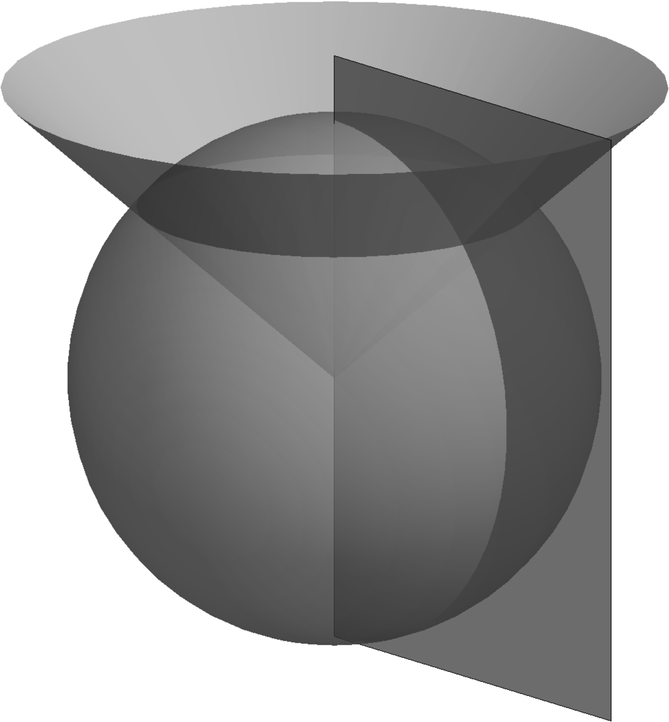 (6.64)
(6.64)This completes our descriptions of the special coordinate systems that will be featured throughout
our narrative.
6.10An attempt at a coordinate-based expression for the gradient
In Chapter 4, we gave a geometric definition for
the gradient of a scalar field , as well as
an alternative definition found in most textbooks, where the gradient is defined as the collection
of the partial derivatives
with respect to Cartesian
coordinates. Having now formally introduced the concept of the coordinate basis for Cartesian coordinates, we may conjecture that the
connection between the two definitions is captured by the equation
that interprets the partial
derivatives as the components of with respect to the coordinate basis
. This identity is indeed correct in Cartesian
coordinates and it is left as an exercise to prove it. However, we must wonder if this relationship
continues to be valid in affine coordinates. Furthermore, we are interested in deriving the general
analytical expression for the gradient that works in all coordinate systems. We will save the
second task for later, but will now show why the above equation does not hold in non-Cartesian
affine coordinates.
In the plane, consider two orthogonal affine coordinate systems. Let the first coordinate system be
Cartesian coordinates corresponding to the
coordinate basis . For the other coordinate system
choose the affine coordinates with the coordinate basis
obtained from by a twofold stretch, i.e.
In other words, in the new, "primed" coordinate system, integer coordinate lines are two Euclidean
units apart. In particular, this means that the primed coordinates are
given in terms of the unprimed coordinates by the equations
Notice that, once again, we are observing coordinates and the associated coordinate bases
transforming by opposite rules.
The two coordinate systems are illustrated side by side in the following figure. The two plots
represent the same scalar field which is, of
course, independent of the coordinates. 
 (6.71)
(6.71)Let denote as a function
of and and denote as a function
of and
.
Importantly, the functions and are different functions.
For example, if
then
Even though the three objects -- the
scalar field along with
the functions and -- are different, it does make
sense to denote them by the same letter due to their
close relationship.
We are now in a position to compare the values of the expressions
Recall that the coordinate basis vectors are related by the equations
In other words, in the change from the unprimed to the primed coordinates, the coordinate basis
vectors double. Thus, the only remaining question is whether the partial derivatives
correspondingly double or halve? We will now show that they, too, double and thus the combined
expression quadruples.
Let us compare the partial derivatives and at a
single point with unprimed
coordinates and primed coordinates . In each coordinate system,
increase the first coordinate by , i.e. consider the point with
unprimed coordinates along with the point with
primed coordinates . These distinct points are illustrated in the
figure above. Observe that the point is
twice as far from as the point
. Thus,
the ratio
is roughly twice as great as
Therefore, in the limit as approaches , we have
Similarly, for the partial
derivatives with respect to the second coordinate, we find
In summary, when we change from the Cartesian coordinates to the affine coordinates
,
both the coordinate vectors and the partial derivatives double. Consequently, the value of
the proposed coordinate expression for the gradient quadruples, i.e.
Thus, we have reach the important conclusion that the value of the expression
depends on the particular choice of
the coordinate system. In particular, it cannot be the coordinate-space representation of the
gradient .
As we mentioned above, this observation makes it clear that a more effective analytical framework
is needed for constructing coordinate-dependent expressions that produce the same value in all
coordinate systems. This task of building such a framework will be accomplished in the next few
chapters. In particular, the correct coordinate-space expression for the gradient will be given in
Chapter 10.
6.11Exercises
Exercise 6.1Calculate for an ellipse with semiaxes and that corresponds to
What is the length of as a function of ?
Exercise 6.2Consider a particle moving uniformly around a circle of radius making a complete revolution in time . Show that its acceleration points towards the center of the circle and has the magnitude , where .
Exercise 6.3Describe the six degrees of freedom in choosing a Cartesian coordinate system in the three-dimensional space.
Exercise 6.4Show that the vectors , , and of a right-handed Cartesian basis satisfy the equations
Exercise 6.5Given two affine coordinate systems and with the respective origins at and and the coordinate bases and related by
show that and are related by a combination of a linear transformation and a shift, i.e.
where are the primed coordinates of .
Exercise 6.6For a scalar field , show that the expression
yields the same vector in all Cartesian coordinates.
Exercise 6.7Furthermore, demonstrate that the expression
corresponds to the gradient of the scalar field as defined in Chapter 4.
Exercise 6.8Show that the expression
yields the same vector in all orthogonal affine coordinates, i.e. affine coordinates characterized by an orthogonal coordinate basis .