Prior to introducing coordinate systems, our main focus had been on the construction of a
geometry-centric approach to Euclidean spaces. Our efforts had yielded valuable insights, but most
of our results were not well-suited for practical calculations precisely due to their geometric
nature. In fact, our experience could have led us to believe that geometric insight and practical
calculations are, to a certain extent, mutually exclusive.
Fortunately, that is not the case. It is the very point of Tensor Calculus to provide an effective
coordinate-based analytical framework that enables practical calculations while preserving
geometric insight. In this Chapter, we will begin to describe that framework and, to this end, we
will begin to shift our focus from the Euclidean space to the associated coordinate
space. In the coordinate space, all vectors are represented by their components and all
other geometric operations (such as the dot product) are represented by systems with scalar
elements (such as the metric tensor). All of the analysis is performed strictly in terms of those
quantities. The advantage, of course, is that, being numerical quantities, such objects are subject
to the robust techniques of Algebra, ordinary Calculus, and computational methods. At the same
time, Tensor Calculus will enable us to continue to think geometrically while proceeding
analytically.
By the components of a vector we, of course, mean its components with respect to the
covariant basis .
Recall, however, that for a general curvilinear coordinate system, the covariant basis varies from
one point to another. In other words, at each point, we find a unique component space that is
different from its neighbors. Thus, the term coordinate space refers to the collection of
the component spaces at all points.
10.1The components of a vector
The covariant basis and
its companion contravariant basis are
equally well-suited for the decomposition of vectors at a given point. Let us first consider the
components of vectors with respect to the covariant basis . These
are known as the contravariant components for reasons that will become obvious shortly.
10.1.1The contravariant components
Denote by ,
, and
, or,
collectively, , the
components of a vector with
respect to the covariant basis , i.e.
With the help of the summation
convention, we write
The summation convention
compelled us to use a superscript to enumerate the components and therefore to use
the term contravariant. As always, this choice will prove to be an accurate predictor of the
manner in which
transforms under a coordinates transformation.
Since the covariant basis varies
from one point to another, one and the same vector decomposed with respect to bases at different
points in the Euclidean space will yield different contravariant components .
Later on, we will provide an analytical method for determining whether two sets of components at
two different points in space represent equal vectors.
With the introduction of contravariant coordinates, note that the almost trivial identity
can now be interpreted in two different ways. On the one hand, it can be seen merely as an instance
of the index-renaming property of the Kronecker delta in a contraction. Alternatively, the
expression on the right can be seen as a linear combination for in
terms of the basis vectors , , and
. Thus,
the elements of the Kronecker delta can also be interpreted as the collection of the contravariant
components of the elements of a basis with respect to itself.
10.1.2The covariant components
When a vector is
decomposed with respect to the contravariant basis , i.e.
the resulting coefficients are
known as the covariant components.
Naturally, the contravariant components and
the covariant components are
closely related and one nearly can guess the relationship between them simply from the placement of
the indices. Recall that the covariant and the contravariant bases are related by the identity
Substituting this relationship into
the expansion , we
find
Thus, since is also
given by , we
have
Equating the coefficients, we arrive
at the relationship between and
, i.e.
Since the metric tensor is
symmetric, i.e. , we
can write this identity in the more pleasing way
Deriving the inverse relationship
in similar fashion is left as an exercise. Alternatively, this relationship can be derived from
by inverting the metric tensor, as described in Section 9.5.2.
Finally, we note that the relationship between the contravariant and covariant components of a
vector, captured by the identities
and
is exactly the same as the
relationship between the covariant and contravariant bases. These relationships are examples of
index juggling which is the subject of Chapter 11. Note that objects related by index juggling are, in fact, so closely
related that we will tend to think of them as two different manifestations of the same object.
10.1.3Various methods for calculating the components
The equations  (10.10)
and
define the components but do not indicate how to calculate them. Depending on the
situation, a practical calculation can be accomplished in a number of ways. In a pure geometric
context illustrated in the two-dimensional figure below, one can construct a parallelogram with
sides parallel to and
and a
vertex at the tip of . Then the
signed ratios of the lengths of the sides of the parallelogram to the lengths of the corresponding
covariant basis vectors are
the contravariant components .
(10.10)An alternative approach is based on decomposition by the dot product. First discussed in Section 2.4, it become our most frequently used approach thanks to its
algebraic nature. We will revisit this method later in this Chapter where it will find a
particularly elegant expression in the tensor notation.
Note that the two methods have a crucial feature in common: each works in any coordinate systems
and each can be described exclusively in terms of quantities available in the context of the chosen
coordinate system. This shared aspect of the two approaches is essential to the concept of a
variant to which we now turn.
10.2The concept of a variant
The covariant and contravariant bases and
, the
contravariant and covariant components and
, and
all other objects introduced in the previous Chapter are examples of variants. We will now
explain the meaning of this important term.
The definition of reads
The very fact that it contains an
explicit reference to the coordinates
points to its dependence on the choice of the coordinate system. Indeed, this is so: the covariant
basis, at a fixed point in space, varies from one coordinate system to another. Objects that
have this property are called variants, subject to an additional requirement described in
the next paragraph. Clearly, any combination of variants -- be it a sum, a product, or the result
of differentiation -- is a variant in its own right. Note, however, that the term variant
refers to the potential to vary from one system to another and is not a guarantee of
variability. Some special combinations of variants, such as , have
the same value in all coordinate systems. Such variants, which are the central objects of our
study, are known as invariants and are described in the next Section.
Importantly, the concept of a variant carries an additional requirement: in order to be considered
a variant an object must be constructed by the same algorithm in all coordinate systems.
This definition is admittedly rather informal and we will therefore attempt to clarify it by
illustrating why each of the objects introduced in the previous Chapter are indeed variants.
Let us start with the covariant basis. To confirm that it is a variant, let us translate its
analytical definition
into words, i.e. in order to
construct the covariant basis ,
differentiate the position vector with
respect to the coordinate . This
algorithm is the same in all coordinates and therefore is a
variant. For the covariant metric tensor ,
note that it is constructed in two steps: 1) construct the covariant basis and 2)
calculate the pairwise dot products .
Thus, is a
variant. The contravariant metric tensor
includes the additional step 3) find the matrix inverse of .
Thus, it is also a variant. Similarly, the contravariant basis needs
a further step 4) evaluate the contraction . Finally, the contravariant
components of a
vector require two
steps: 1) construct the covariant basis and 2)
decompose with
respect to .
The dependence of a variant on the coordinate system may be likened to the dependence of length on
the units of measurement. For example, the length of a segment may be described as centimeters in the metric system or as inches in the imperial system. Meanwhile, the length of
a segment is, of course, a valid concept that exists in the absence of any system of measurements.
Therefore, a specific value of length in a particular measurement system can be thought of as a
manifestation of length in that system. Similarly, a variant may be thought of as an
entity that exists outside of any coordinate system, while the specific set of values that
represent it in a particular coordinate system may be thought of as its particular coordinate
manifestation. Thus, we can identify a variant with the algorithm that produces it, such as
differentiation of the position vector with respect to coordinates for the covariant basis.
A variant, having different values in different coordinate systems, is said to transform
from one coordinate system to another. Of great interest to us will be the transformation
rule, i.e. the equation that relates the values of a variant in the different coordinate
systems. We will discover that some variants, which we will call tensors, are subject to a
particularly transformation rules. As you may expect, these special variants will play an
instrumental role in our subject.
Finally, note that at this point, we would be hard-pressed to think of an object that is not
a variant. We will encounter our first non-variant in Chapter 13 when we introduce the Jacobian which requires the presence of two
coordinate systems.
10.3The concept of an invariant
The covariant basis and
the contravariant components of a
vector are
variants. Thus, by definition, the contraction
is also a variant. However, it is a
very special kind of variant: it has the same value, namely the vector , in all
coordinate systems. Such a variant is called an invariant.
Invariants, by virtue of their independence from the choice of coordinates, are the ultimate
objects of our study. Above all, the purpose of Tensor Calculus is to study the natural world (or,
at least, a geometric idealization of it). Thus, every meaningful analysis must ultimately yield
objects that are independent of coordinates.
Of course, the statement that the combination is
independent of coordinates is nearly tautological since the components are
constructed precisely in such a way as to produce by the
contraction . Going
forward, we will encounter invariants that arise in far more nontrivial ways. Nevertheless, the key
to invariance will be exceptionally simple: the expression must be comprised of tensors and have
all indices contracted away.
The combination also
offers an insight into the eventual meaning of the terms covariant and contravariant
as applied to tensors, i.e. variants subject to a special transformation rule -- or, to be more
precise, one of two rules that are the inverses of each other. One of the rules is called
covariant and the other -- contravariant . Covariant tensors transform in the
same way as the basis --
thus co. Contravariant tensors transform in the opposite way -- thus contra. When two
objects that transform according to opposite rules are combined, the two transformations cancel
each other and, as a result, the value of the combination in one coordinate system equals its value
in the other coordinate system. In other words, the combination is an invariant. This, in a
nutshell, is how invariants are produced in Tensor Calculus.
10.4Decomposition by the dot product, revisited in the tensor notation
In Section 2.4, we considered the decomposition of a vector
with
respect to a basis .
Recall that the components of , which we
at the time denoted by , were
given by the equations
for an orthonormal, a.k.a.
Cartesian, basis ,
for an orthogonal basis , and
for an arbitrary basis .
We will now switch to the covariant basis and
the contravariant components . Note
that replace with
and
with
in
the above equations yields identities that are invalid from the tensor notation point of view, i.e.
U^{i} & =mathbf{Z}_{i}cdotmathbf{U,}tag{} U^{i} &
=frac{mathbf{Z}_{i}cdotmathbf{U}}{mathbf{Z}_{i}cdot mathbf{Z}_{i}},text{ and }tag{} left[ begin{array} {c} U^{1} U^{2} U^{3} end{array}
right] & =left[ begin{array} {ccc} mathbf{Z}_{1}cdotmathbf{Z}_{1} &
mathbf{Z}_{1}cdotmathbf{Z}_{2} & mathbf{Z}_{1}cdotmathbf{Z}_{3} mathbf{Z}_{2}cdotmathbf{Z}_{1} &
mathbf{Z}_{2}cdotmathbf{Z}_{2} & mathbf{Z}_{2}cdotmathbf{Z}_{3} mathbf{Z}_{3}cdotmathbf{Z}_{1} &
mathbf{Z}_{3}cdotmathbf{Z}_{2} & mathbf{Z}_{3}cdotmathbf{Z}_{3} end{array} right] ^{-1}left[
begin{array} {c} mathbf{Z}_{1}cdotmathbf{U} mathbf{Z}_{2}cdotmathbf{U} mathbf{Z}_{3}cdotmathbf{U}
end{array} right] .tag{} end{align} Recall from Section 9.5.4, that the matrix above
corresponds to the covariant metric tensor .
Therefore, its inverse corresponds to the contravariant metric tensor .
Despite its invalid form, the equation
U^{i}=mathbf{Z}_{i}cdotmathbf{U}
tag{} end{equation} is correct for an orthonormal
basis ,
although it is, of course, limited to that special case. This is observed for most equations that
violate the rules of the tensor notation: they are typically correct only in a narrow range of
special cases.
Crucially, the notational flaw in the above equation is easily fixed by replacing the covariant
basis with the contravariant basis, i.e.
In words: the contravariant
component of
the vector is given
by the dot product of with the
contravariant basis vector . This
equation remains valid for an orthonormal basis since,
in that case,
coincides with .
However, somewhat remarkably given its utmost simplicity, this equation is valid for an
arbitrary basis . In
other words, it is valid in all coordinate systems.
To observe why this is so, note that the equation
in matrix terms reads
Thus, it can be seen that the
equation
is simply the tensor form of the
equation
which is valid for an arbitrary
basis .
The remarkably simple equation
can also be derived quite concisely
by pure tensor means. Simply dot both sides of the equation
with , i.e.
Since and
, we
have
or
as we set out to show.
Note that the simplicity of the equation
does not imply that the matrix
inversion inherent in linear decomposition can be circumvented. Instead, this equation hides the
inversion in the contravariant basis and,
in doing so, organizes the decomposition algorithm with respect to an arbitrary basis in such a way
that it appears as simple as for an orthonormal basis.
It is left as an exercise to show that the covariant components are
given by the individual dot products with the elements of the
covariant basis, i.e.
The remarkable compactness of these identities is a testament to the tensor framework. While
economy of notation does not imply economy of computation, the expressive power of the tensor
notation is undeniable as it represents the best of two worlds: tensor expressions are as simple as
those associated with Cartesian coordinates yet are valid in all coordinate systems. This pattern
is found throughout Tensor Calculus, and we are about to see it again in our discussion of the
coordinate space representation of the dot product.
10.5The dot product in the coordinate space
In Section 2.6, we established the expression for the dot
product of two vectors in terms of their components. Specifically -- once again switching to the
symbols ,
, and
-- we
showed that the dot product is given by the matrix equation
If the matrices
corresponding to and
are
denoted by and , and once again
denotes the matrix corresponding to ,
then is given by
If the basis is orthonormal,
and therefore is the
identity matrix, then the dot product reduces to the classical form
You have probably already guessed that the tensor equivalent of is .
In fact, we have already essentially derived it in the tensor notation in Section 8.4. However, since the derivation fits on a single line, we
are happy to repeat it here. Recall that
In the second equation, rename the
index into , i.e.
in preparation for using the two
contractions in a single expression. Now, dot both sides of the equations above, i.e.
and note the chain of identities
Thus, we have arrived at the
fundamental identity
This crucial identity clarifies the
meaning of the term metric in metric tensor: the metric tensor is used for evaluating
dot products, and therefore lengths and angles, in the Euclidean space.
In terms of the underlying arithmetic operations,
is equivalent to the matrix expression and it nearly matches its
compactness. In addition, it is indifferent to the order of the multiplicative terms and lacks the
need for the transpose. Furthermore, the expression
is subject to further "compactization". Recall that the combination
yields the covariant component .
Therefore, the equation
can be rewritten in the form
or, by the same token, in the form
Note that in the unpacked form, the
last equation reads
which clearly demonstrates that we
have been able to achieve the simplicity of the classical Cartesian expression found in the
equation
from Chapter 2. Meanwhile, the equation
is valid in all bases. Its
simplicity speaks to the expressive power of the tensor framework.
Finally, note that the length of a vector in
component form is given by
which can be expressed more
compactly as
10.6The dot product in special coordinate systems
Although the equation
along with its unpacked form
is valid in all coordinate systems,
it will be useful to document the explicit expressions in standard coordinate systems corresponding
to the equation
that expresses the dot product in
terms of the contravariant coordinates only.
In Cartesian coordinates, the covariant metric tensor is represented by the identity matrix and
therefore
In other words,
In polar coordinates in a two-dimensional space,
and, therefore, is given by
In cylindrical coordinates,
and, therefore, is given by
Finally, in spherical coordinates,
and, therefore, is given by
10.7The natural association between geometric vectors and first-order systems
With every geometric vector , we
associate its contravariant components . This
association works in both directions: from the vector, we can determine the components, and from
the components, we can reconstruct the vector. Furthermore, we can naturally associate the vector
with
any first-order system with
scalar elements, regardless of how the system may have arisen.
Thus, there is a natural one-to-one correspondence between first-order systems and geometric
vectors. In fact, this correspondence is so strong that we may go as far as referring to
first-order systems as vectors. That is, we may write consider a vector
instead of consider a vector with components . In
other words, in the context of Euclidean spaces, a vector and its components are so closely linked
that the terms vector and components of a vector become interchangeable.
10.8The components of the velocity of a material particle in motion
In order to demonstrate how a practical analysis may be conducted in the component space, let us
analyze the motion of a material particle in a Euclidian space. Suppose that the Euclidean space is
referred to an arbitrary coordinate system and
that the trajectory of the particle is given by the equations
where represents time. The functions are referred to as the equations of the
motion.
Let our goal is to express the components of
the particle's velocity vector and the components of
the acceleration vector in terms of
the equations of the motion . Note that at each point along the
trajectory, the vectors and must be
decomposed with respect to the covariant basis found
at that point.
In this Section, we will show that the velocity components are
given by the intuitive equation
Meanwhile, the equation for the
acceleration components will
be postponed until later since it requires the introduction of the Christoffel symbol
which is the subject of Chapter 12.
We described the equation
as intuitive since it can be
easily seen to be true in an affine setting. Indeed, in affine coordinates, the position vector
along the
trajectory is given by the function
provided that emanates
from the origin of the coordinate system. In other words, the functions represent the components of with respect to the constant basis . Differentiating both sides with respect to , we find that
which leads to the conclusion that
the velocity components are
given by
However, it is clear that the above
derivation is limited to affine coordinates since it assumes that the coordinate basis does not
vary with . Thus, the fact that the equation
remains valid in curvilinear
coordinates is perhaps somewhat unexpected.
Let us now derive the equation
in general curvilinear coordinates.
Start with the definition of the velocity , i.e.
where represents the values of the position vector
along the trajectory. The function can be formed by composing the function , i.e. the position vector a function of the
coordinate , with
the equations of the motion . In other words,
By the chain rule, we find
Since the derivative
yields the covariant basis , we
have
Therefore, the derivatives
are indeed the contravariant
components of
, i.e.
as we set out to show.
Two surprising aspects of this identity that are worthy of note. First is the very fact that it is
true despite the spatial variability of the covariant basis. As we show below, the analogous
equations for the acceleration components , i.e.
A^{i}=frac{dV^{i}left( tright)
}{dt} tag{} end{equation} or, equivalently,
A^{i}=frac{d^{2}Z^{i}left( tright)
}{dt^{2}}, tag{} end{equation} do not hold -- precisely due to the
variability of the basis.
The second surprising aspect of the equation
is the fact that it does not
reference either the position vector or the covariant basis or any other geometric elements of the
Euclidean space. Meanwhile, one and the same equations of motion
describe completely different
trajectories in different coordinate systems. For example, the equations
describe a parabola in Cartesian coordinates and a spiral in polar coordinates. Thus, the two
motions are characterized by completely different velocity vectors . Nevertheless, the components of
the velocity, i.e.
are the same for both motions.
10.8.1Example: Uniform motion along a helix
For a specific example, consider a particle moving along a helix in a three-dimensional Euclidean
space. If the Euclidean space is referred to cylindrical coordinates oriented in a natural way with
respect to the helix, then the equations of the motion read
where is the radius
of the helix, is the
angular velocity of the circular motion, and is the span
of the helix. Therefore, the components of the velocity, given by the equation
have the following constant
values
Of course, even though the components of the velocity vector are constant, the velocity vector
itself is variable due to the variability of the accompanying basis.
The magnitude of the
velocity can be calculated by the formula
Along the helix, this formula reads
and therefore
Thus,
It is left as an exercise to the
repeat this calculation in Cartesian coordinates.
10.8.2A note on the components of acceleration
As we have already stated, the components of
the acceleration vector do not
equal the time derivative of the components of
the velocity vector, i.e.
If nothing else, this is clear from
the example of uniform motion along a helix that we analyzed in the previous Section. Since the
components of
the velocity vector are constant, their derivatives vanish, i.e.
Meanwhile, the acceleration of the
particle moving along a helix is not zero and therefore .
The underlying reason for the failure of the formula
is, of course, the spatial
variability of the covariant basis. In order to establish the correct relationship, let us
once again start our analysis with a geometric object: the acceleration vector , defined as
the derivative of the velocity vector , i.e.
Since is given by the equation
where is a function that represents the covariant
basis along
the trajectory, differentiating the above equation yields
This is the crucial moment. The
second term does not vanish since the derivative
represents the (nonvanishing) rate
of change of the basis vector along
the trajectory. As a result,
and consequently
Therefore, in order to advance our
analysis further, we must tackle the spatial variability of the covariant basis. This line of
inquiry, which leads to the concept of the Christoffel symbol, is developed in Chapter 12.
10.8.3The components of the tangent vector to a curve
The analysis similar to that of the motion of a material particle can be applied to abstract
geometric curves. Consider a curve parameterized by a generic variable rather than time . In terms of the , the equations of the curve
read
Based on our foregoing discussion,
we can conclude that the derivative
represents the contravariant
components of a tangent vector.
Suppose now that the curve is parameterized by arc length , i.e.
In Chapter 5, we established that the derivative
produces a unit tangent . Thus, the
contravariant components of
the unit tangent are given
by the equation
The fact that is unit
length is expressed in terms of its components by the equation
or, equivalently,
10.9The arc length integral in the component space
In Section 5.2, we considered a curve given by the vector
equation
where is an arbitrary parameter along the
curve. We showed that the arc length of the segment between the points
corresponding to values and
of the
parameter is given by the integral
On the one hand, this formula, which
does not require coordinates in the ambient space, proved to be of great theoretical value. On the
other hand, due to the lack of ambient coordinates, this formula cannot be used for practical
calculations of the length of any concrete curve since it features geometric quantities rather than
algebraic expressions. However, since we have introduced coordinates in the ambient space and are
now able to work with the components of vectors, we can modify the above formula in order to make
it suitable for practical calculations.
Introduce an arbitrary coordinate system in
the ambient Euclidean space and let the equations of the curve read
As we demonstrated in the previous
Section, the derivative is given by the equation
In other words,
are the contravariant components of
. Since the dot product of a vector with itself
is given by the formula
we have
With the help of this identity, the
equation
becomes
Let us once again stress one of the most crucial aspects of this formula: it is valid in
arbitrary coordinates as
well as for an arbitrary parameterization of the curve, provided that
. The
practical advantage of this formula over the coordinate-free equation
is overwhelming and speaks to the
immense utility of coordinate systems.
For a concrete example, let us calculate the arc length of a complete loop of the spiral in the
following figure. The spiral can be described geometrically as a locus of points whose distance
from a particular point equals the
angle, in radians, to a reference ray . Notice that
the distance from to the point
where the spiral intersects the reference line for the first
time is .  (10.80)
Evaluating the length of this curve in a coordinate-free setting would present a formidable
challenge. With the use of coordinates, however, this task becomes a routine exercise in ordinary
Calculus. Let us perform the required analysis in two alternative ambient coordinate systems:
Cartesian coordinates and polar coordinates
.
(10.80)
Evaluating the length of this curve in a coordinate-free setting would present a formidable
challenge. With the use of coordinates, however, this task becomes a routine exercise in ordinary
Calculus. Let us perform the required analysis in two alternative ambient coordinate systems:
Cartesian coordinates and polar coordinates
.
(10.80)First, introduce a Cartesian coordinate system that lines up with the
reference line as in the
following figure.  (10.81) The equations of the curve that
describe the spiral in these coordinates read
(10.81) The equations of the curve that
describe the spiral in these coordinates read
(10.81)
Since, in Cartesian coordinates, the metric tensor at
all points corresponds to the identity matrix, we have
The derivatives and are given by
and therefore the integrand is given by
Thus the arc length is given by the ordinary integral
A routine evaluation of the integral
yields the final answer
Now introduce the polar coordinate system , where the origin of the coordinate
system coincides with the point and the polar
axis coincides with the ray . In these
coordinates the equations of the curve take on a particularly simple form, i.e.
Recall that the metric tensor
corresponds to the matrix
Along a general curve given by the
equations and spiral, corresponds to the matrix
Thus, for a general curve in polar
coordinates, the integrand is given by
For our specific curve, corresponds to
Since derivatives and are given by
the integrand is given by
Not surprisingly, we obtained the
exact same expression for the integrand since it equals the length of the vector and does not depend on the choice of the
ambient coordinates. Thus, the rest of the analysis can proceed as before.
This simple examples illustrates the great advantage of the coordinate space approach as it enables
us to convert geometric expressions into arithmetic ones which can then be evaluated by the robust
techniques of ordinary Calculus.
10.10Computing the metric tensor from lengths of curves
The equation
demonstrates that, in combination
with the equations of the curve, the metric tensor gives us the ability to calculate the length of
any curve. In other words, we do not need any additional geometric details regarding either the
curve or the coordinate system.
Crucially, this connection between the metric tensor and the lengths of curves also works in the
opposite direction. Namely, an ability to measure the lengths of curves can be used to calculate
the metric tensor. Thus, any quantity that can be calculated solely from the metric tensor (and its
derivatives) can, in fact, be calculated from the very narrow ability to measure the lengths of
curves. This insight will have important implications in the study of Riemannian spaces which we
will undertake in Chapter 20.
Let us begin by calculating the entry at a
fixed point with coordinates . Consider the coordinate line corresponding to
the coordinate
illustrated below in a two-dimensional figure.  (10.99) The equations of this coordinate line read
(10.99)
For a positive , denote the length of this curve from
the point to the point with coordinate by . Importantly, the assumption that we are able
to measure the lengths of curves by some means (perhaps by taking measurements with the help of
some mechanical device) implies that the function is available -- meaning that we can evaluate
its values and the values of its derivatives.
Since is the only function in the equations of the
curve that varies with , the only surviving term in the sum
is
Therefore, is given by the integral
By the Fundamental Theorem of
Calculus, the derivative equals the integrand at , i.e.
Thus, the element of the
metric tensor at the point is given by the formula
Thus, we have demonstrated a way to
calculate from
the lengths of curves. The same approach can be used to evaluate other "diagonal" elements and
of
.
To calculate the "off-diagonal" elements, say ,
consider the curve given by the equations
Since the derivatives are
we have
and therefore
Therefore, the derivative of at the point is given by
Since the diagonal terms and
are
already available, we are able to compute
according to the formula
The remaining off-diagonal entries
can be calculated in similar fashion.
10.11Coordinate space expressions for the directional derivative and the gradient
Recall from Chapter 4 that the direction
derivative is defined as the rate of change in
along the ray
. 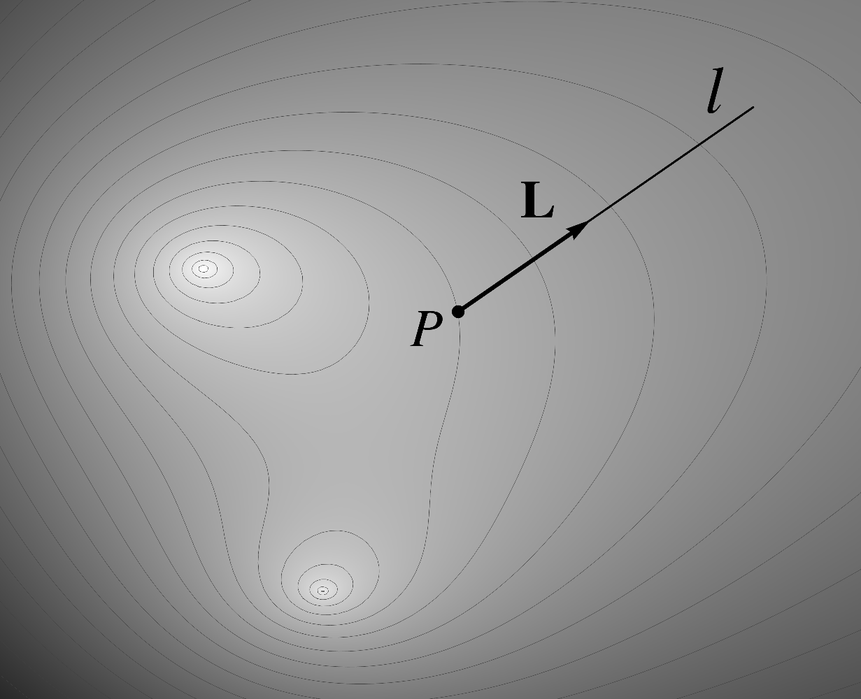 (10.118) For a scalar field , we
demonstrated that is given by the equation
(10.118) For a scalar field , we
demonstrated that is given by the equation
(10.118) where is the unit
vector that points in the direction of the ray and the
vector is the gradient of . In this
Section, we will derive the coordinate space expression for the directional derivative which will,
in turn, yield the coordinate space expression for the gradient.
Let be
the contravariant components of , i.e.
Suppose that the ambient space is
referred to arbitrary coordinates and
that the equations of the ray when
parameterized by arc length read
Note that even though the ray is straight,
the functions are not necessarily linear.
Along the ray, the values of the field form a
function of denoted by . By definition, the directional derivative
along the ray equals with
, i.e.
Observe that the function can be obtained by composing the function
, i.e. the dependence of on the
ambient coordinates , with
the equations of the curve , i.e.
Differentiating both sides, we find
The collection of partial derivatives
will prove to be a dominant object
in our narrative and therefore deserves its own symbol with a clearly indicated index placement.
Thus, we will denote it by , i.e.
In Chapter 15, the symbol will
be extended to the new differential operator known as the covariant derivative.
Meanwhile, as we described in Section 10.8.3, the
derivatives
represent the components of the unit
tangent to the ray , which is
precisely the vector . Therefore,
we have
In summary, the directional
derivative is captured by the equation
which constitutes the coordinate
space representation of the directional derivative. As with all other coordinate space formulas
that we have encountered so far, it is valid in all coordinate systems.
The formula
will now reveal to us the coordinate
space representation of the gradient, which has eluded us until now. The combination
represents the dot product of the two vectors
The second vector is, of course,
. Since the
formula
holds for every unit vector , we can
conclude that the combination must
represent the gradient , i.e.
This is the coordinate space
representation of the gradient that we have been seeking ever since
Chapter 4.
We can now understand the underlying flaw in our original attempt at the coordinate space
expression for the gradient, i.e.
found at the end of Chapter 6. In more general terms, this equation may be
rewritten as
or, equivalently,
mathbf{nabla}F=nabla_{1}F
mathbf{Z}_{1}+nabla_{2}F mathbf{Z} _{2}+nabla_{3}F mathbf{Z}_{3}. tag*{} end{equation} With the help of the summation sign, it
can also be written as
Naturally, we cannot write this
expression without the summation sign since the combination
violates the rules of the tensor notations that require the repeated indices to be of opposite
flavors in a contraction. Correspondingly, we observed in Chapter 6 that when a coordinate system is "stretched" by a factor , both and double
and thus the product
quadruples. In other words, the above formula produces different vectors in different coordinate
systems and is therefore -- to put it bluntly -- geometrically meaningless.
Although we have not yet studied transformation of variants under coordinate changes, we can rely
on the tensor notation in order to predict the reason why the sum
quadruples. Both elements in the product have subscripts and therefore transform in the same way
under a change of coordinates. Thus, if
doubles then so does and then their product,
predictably, quadruples. The formula
by combining objects that transform
by opposite rules, corrects our original mistake.
Interestingly, our original guess that the components of the gradient of are the
partial derivatives
was correct. What we have originally
missed, but have now corrected, was to interpret those values as the covariant components
that must be combined with the contravariant basis.
10.12The shift to the coordinate space way of thinking
We started our overall narrative in a strictly geometric setting with the geometric vector
being the primary object of our study. There were several advantages to such an approach. First, it
enabled us to lean heavily on our geometric intuition. Second, it allowed us to develop an
analytical framework characterized by a very limited number of available operations. Finally, we
were able to use the geometric space as an absolute reference, which enabled us to assure the
internal consistency of our calculations.
On the other hand, what our approach lacked was the capability to analyze specific problems. We
have now addressed this shortcoming by switching to the analysis of the components of vectors
rather than the vectors themselves. Several examples in this Chapter have already demonstrated the
great utility of this coordinate space approach. What is particularly appealing about it is
that it is not a replacement but an augmentation of the geometric approach. Thus, our
geometric framework will continue to provide us with an opportunity to verify our results in the
geometric space. However, our emphasis will begin to shift towards the component perspective.
10.13Exercises
Exercise 10.2Derive the equation
from the equation
Exercise 10.3In spherical coordinates, find the contravariant and the covariant components and of the unit vector pointing in the direction of the polar axis at a point with coordinates . Confirm that .
Exercise 10.4Analyze the helical motion described in Section 10.8.1 in Cartesian coordinates. Namely, find the contravariant components of the velocity vector for a particle moving along a helix. Confirm that the resulting expression for the magnitude of the velocity vector is the same as found in Section 10.8.1.