Having laid down the algebraic foundations of geometric vectors, we now turn our attention
to differentiation. When most people think of differentiation of vectors, they imagine a
component-by-component operation, such as . This way of thinking is an example of the
presumptive association between geometric vectors and their components. It is imperative to break
this association and to commit to vectors as geometric objects. As we are about to demonstrate,
geometric vectors in a Euclidean space have just enough analytical structure to be meaningfully
differentiated. Differentiation of geometric vectors will prove to be a crucial element in our
approach to Tensor Calculus.
4.1The mechanics of differentiation
Recall the standard definition of the derivative of an ordinary function , i.e.
What is required of in order for this definition to apply?
Clearly, the quantity represented by must be subject to three basic operations:
addition, multiplication by numbers, and evaluation of limits. Addition (which implies subtraction)
is required in order to evaluate the difference . Multiplication by numbers (which implies
division) is required in order to divide the difference by . Finally, the need for limits is
self-evident.
We have already established that geometric vectors can be added and multiplied by numbers. Thus, we
only need to confirm that geometric vectors are subject to evaluation of limits. What makes limits
of geometric vectors possible is the availability of Euclidean length since it enables us to state
how close two vectors are by measuring the distance between them. The distance
between two vectors and , denoted by , is defined as the length of their
difference, i.e.
With the distance function in hand,
we are able to carry the classical definition of a limit over to geometric vectors.
In formal terms, a vector is the
limit of a sequence if the
distance between and
approaches
as approaches infinity, i.e.  (4.4) The same approach can be used to define the limit of a
vector-valued function . Specifically, the vector is the
limit of at if the
distance between and approaches
as approaches , i.e.
(4.4) The same approach can be used to define the limit of a
vector-valued function . Specifically, the vector is the
limit of at if the
distance between and approaches
as approaches , i.e.
The following figure illustrates a
sequence of vectors that
approach the "vertical" vector .
(4.4) Thus, the concept of a limit for
vector-valued sequences and functions is established.
Having established the concept of a limit, we can mimic the classical definition
of the derivative to give a formal
definition of the derivative of a vector-valued function that, i.e.
We reiterate that all aspects of the
procedure encoded in this definition can, at least conceptually, be carried out by pure geometric
means without the use of a coordinate system.
The derivative of a vector function corresponds to our intuition for rate of change, except
now the rate of change is a vector quantity. Nevertheless, many of the ideas from ordinary
Calculus carry over to vector-valued functions. For example, the derivative can be used for linear
approximations. Namely, for a small , the derivative can be approximated by the quotient
in the sense that the
distance between and the above quotient is small. Therefore,
can be approximated by the
familiar formula
also in the sense that the
distance between and is small.
4.2The derivative of a vector function as the tangent to a curve
A vector-valued function has the inescapable geometric
interpretation as the curve traced out by the tips of the vectors emanating from a single point known as the
origin. In this context, the vectors are referred to as the position
vectors for the points on the curve. Since it is common to denote position vectors by the
letter rather than
, we will
now switch to that convention and consider a vector-valued function and refer to it as the vector equation of
the curve.  (4.9)
(4.9)
(4.9)To reiterate: there is a natural one-to-one correspondence between vector-valued functions and
curves. Any vector-valued function can be visualized as a curve with respect to
a fixed origin . Conversely,
every curve represents a vector-valued function once a fixed origin is chosen and
a numerical value of a parameter is assigned to every point on the
curve in an appropriate fashion. If the parameter represents time, then the curve
associated with the function can be interpreted as a trajectory of a
moving particle.
Given this interpretation of a vector-valued function , what is the meaning of the vector ? We will now demonstrate is a vector that points in the
tangential direction to the curve. We intuitively understand the tangent line to be a
straight line that "touches" the curve at a single point, typically without crossing it.
Alternatively, we can think of the tangent as the straight line that presents itself when one
sufficiently zooms in on the curve. Our present goal is to confirm that the definition of is consistent with our intuition for the
tangent line. We will do so by examining the limiting procedure encoded in the analytical
expression for , i.e.
Once our intuition is confirmed, we
will reverse the logic and define the tangent direction as the direction of the vector . Additionally, if is interpreted as the trajectory of a
particle, where represents time, then the
velocity of the particle will be defined to be .
The following figure shows for two points corresponding to two nearby
values and of the
parameter.  (4.11) The difference is the vector from the tip of to the tip of .
  (4.12) Importantly, note that the difference is independent of the location of the origin
. This is why
the location of is almost
always irrelevant. If is thought of as time, corresponds to the displacement of the
particle over the short period of time .
(4.12) Importantly, note that the difference is independent of the location of the origin
. This is why
the location of is almost
always irrelevant. If is thought of as time, corresponds to the displacement of the
particle over the short period of time .
(4.11)(4.12)Dividing the difference by yields our initial approximation to the
eventual vector .  (4.13) When is thought of as time, the ratio
(4.13) corresponds to the average
velocity of the moving particle over a period of time .
Finally, imagine what happens to the vector represented by the above ratio as begins to approach zero, and observe that its
direction begins to approach what we intuitively understand as the tangent to the curve.  (4.15) Thus, we have justified the interpretation of the derivative
of a vector-valued function as the tangent to the curve represented by
.
(4.15) Thus, we have justified the interpretation of the derivative
of a vector-valued function as the tangent to the curve represented by
.
(4.15)4.3Differential analysis of the unit circle
Having gained this important insight, let us determine for a specific curve that will prove to be of
great importance in our future investigations. Suppose that traces out the unit circle where the
parameter corresponds to the central angle
measured in the counterclockwise direction with respect to an arbitrary ray emanating from the
center of the circle.  (4.16) Since, as we remarked previously,
is independent of the location of the origin
, let us place
it at the center of the circle. We have already established that is tangential to the circle and it is evident
that it points in the counterclockwise direction. Thus, the only remaining quantity to be
determined is its length.
(4.16) Since, as we remarked previously,
is independent of the location of the origin
, let us place
it at the center of the circle. We have already established that is tangential to the circle and it is evident
that it points in the counterclockwise direction. Thus, the only remaining quantity to be
determined is its length.
(4.16)If we think of as time and the unit circle as the
trajectory of a material particle corresponding to , then it is clear that is unit length. Indeed, as changes from to , the particle makes a single
revolution and thus travels a distance of . Therefore, its speed, i.e. the
magnitude of , has the constant value of  (4.18)
In other words, is a unit tangent vector that points in the
counterclockwise direction.
(4.18)The same conclusion regarding the magnitude of can be reached by a more formal calculation.
Consider the configuration involving and for two nearby values of the
parameter.  (4.19) From the isosceles triangle with the
vertices at , , and , we calculate that
(4.19) From the isosceles triangle with the
vertices at , , and , we calculate that
(4.19) and therefore
From ordinary Calculus, we know that
Therefore,
and thus is indeed unit length, consistent with the
earlier conclusion based on our kinematic intuition.
Finally, for a circle of radius , similarly
parameterized by the central angle ,  (4.24) the derivative is the tangential vector of length , i.e.
(4.24) Proving this fact is left as an
exercise.
4.4The laws of vector differentiation
Geometric vectors are subject to three operations: addition, multiplication by scalars, and the dot
product. Naturally, to each operation there corresponds its own differentiation rule.
4.4.1The sum and product rules
Consider two vector-valued functions and . The derivative applied to their sum is
governed by the familiar sum rule
For the product of a vector-valued
function with a constant scalar, the differentiation rule reads
If the scalar is itself a function of , then the product rule reads
The proofs of these rules are left
as exercises. While demonstrating the first two identities is entirely straightforward, the last
one may pose a challenge. We recommend applying the same approach that we are about to apply to the
dot product rule.
4.4.2The dot product rule
We will now demonstrate that vector-valued functions satisfy the dot product rule
which is entirely analogous to the
product rule in ordinary Calculus. Not surprisingly, we will also be able to demonstrate this rule
by borrowing an argument from Calculus.
Let
and consider the difference
On the right, subtract the
combination from the first term and add it
to the second, i.e.
By the distributive law,
Divide both sides by , i.e.
Finally, evaluate the limit as approaches zero. By definition, the left side
approach
Meanwhile, the two fractions on the
right approach to and , and approaches . Thus, the right side converges to
leading to the identity
as we set out to show.
4.5The derivative of a constant-length vector function
As one demonstration of the dot product rule, let us show that if has constant length then is orthogonal to . In algebraic terms, the fact that has constant length can be expressed with the
help of the dot product by the equation
where is a constant. An application of the dot
product rule yields
The two terms on the left are equal
and therefore both equal zero. In other words, the dot product of and vanishes
In other words, is indeed orthogonal to .
Orthogonality between and for a constant-length function can also be derived from the previously
observed fact that is tangential to the curve traced out by
when the vectors emanate from a fixed point . When the
vectors represented by a constant-length function are arranged in such a way, the tips of trace out a circle, although not necessarily
in a constant-speed fashion encountered in the previous Section. Since is tangential to the circle, it must be
orthogonal to as the latter points in the radial direction.
For another interesting interpretation of orthogonality between a constant-length vector and its
derivative, imagine a particle moving along a curved path with constant speed. Because the
particle's trajectory is not straight, its velocity is not constant. However, the
magnitude of the velocity, i.e. speed, can remain constant even along a curved
trajectory.  (4.41) As we have established previously, the
velocity vector is tangential to the trajectory. Its
derivative , which is orthogonal to , is the acceleration . Thus, the fact established in this Section
shows that the acceleration of a particle moving with constant speed is orthogonal to the
trajectory.
(4.41) As we have established previously, the
velocity vector is tangential to the trajectory. Its
derivative , which is orthogonal to , is the acceleration . Thus, the fact established in this Section
shows that the acceleration of a particle moving with constant speed is orthogonal to the
trajectory.
(4.41)We will now turn our attention to the important concepts of the directional derivative and the
gradient of a scalar field.
4.6The directional derivative
A field is a quantity defined at every point of a domain in a Euclidean space. We will
consider fields of scalar, vector, and (eventually) variant quantities. An example of a
scalar field is the temperature distribution in a room. The following figure shows a density
plot of a two-dimensional scalar field, where the color of a given point corresponds to the
value of the field. Meanwhile, the plotted contours, known as level sets, corresponds to a
particular fixed value of the function defining the field. 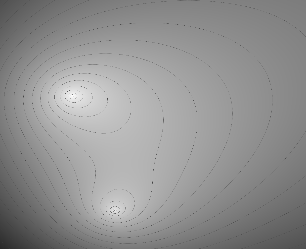 (4.42)
(4.42)An example of a vector field is the distribution of velocities in a fluid flow. A vector field is
usually represented by plotting the vectors of the field at a strategic sampling of points.  (4.43)
(4.43)The concept of the directional derivative can be applied to a field of any kind. As the name
suggests, it measures the rate of change of the field in a particular direction.
Consider a scalar field defined in a
Euclidean space. We will now construct its directional derivative at a point in the
direction indicated by a unit vector . Let be the ray
that emanates from the point in the
direction of . The
following figure shows these elements as well as the density plot for . 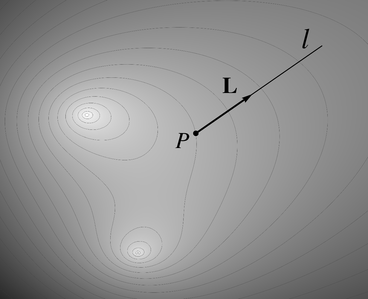 (4.44)
(4.44)For a small positive number , find the point along
whose
Euclidean distance to equals . Denote the values of at the two
points by and . 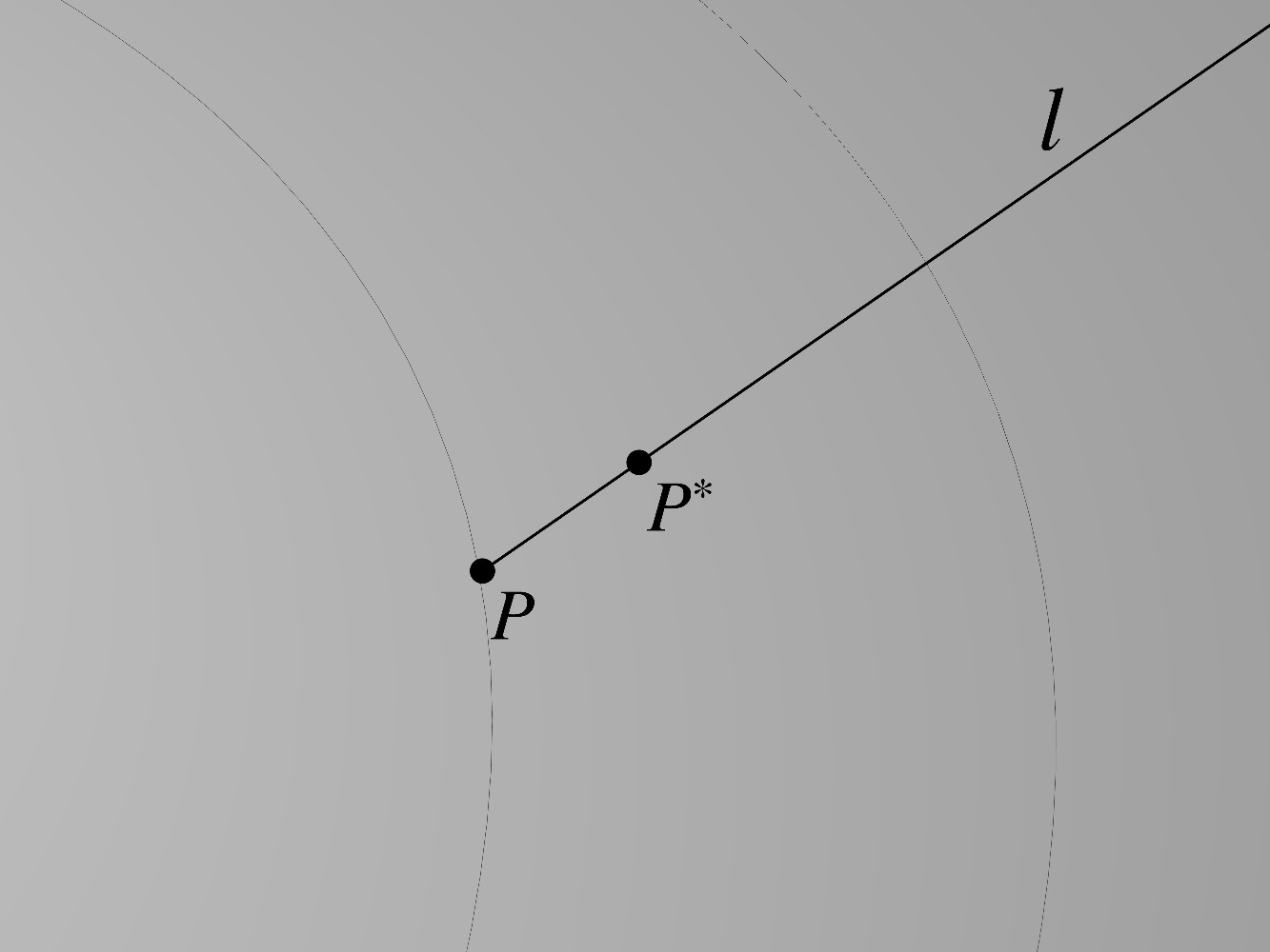 (4.45) The difference represents the change in from to ,
while the ratio
(4.45) The difference represents the change in from to ,
while the ratio
(4.45) can be thought of as the average
rate of change. As approaches , this quantity approaches the instantaneous rate of
change of in the
direction . This
quantity is denoted by and is known as the directional
derivative of in the
direction . In formal
terms,
The same definition can be applied to a vector field textbf{}, i.e.
Note, once again, that vectors are
subject to each of the operations featured on the right side of this equation. Also note that, like
most of the concepts introduced in this book so far, the directional derivative is defined in pure
geometric terms without a reference to a coordinate system.
Rather than directly relying on the concept of a limit, the directional derivative can be defined
in terms of the ordinary derivative. Identify with every point in the Euclidean space the position
vector emanating
from an arbitrary origin so that the
scalar field can be
thought of as a function of the position vector. Denote the position
vector associated with the point by . Then
the expression captures the points along the ray while captures the corresponding values of . Since is a unit
vector, the parameter represents the distance to the point . Thus, the
directional derivative can be defined as the ordinary
derivative of with respect to , i.e.
Naturally, the same idea applies to vector fields. For a vector field textbf{}, consider
the vector-valued function textbf{} and define textbf{} as the derivative with respect to
of textbf{}.
4.7Directional derivative examples
Let us now consider several examples involving the directional derivative. In addition to serving
as concrete illustrations of the concept, these examples will offer two further benefits. First,
they will reinforce the pure geometric nature of our narrative. Second, they will yield results
essential for a number of future applications, including the introduction of the covariant basis in
Chapter 9 and of the Christoffel symbol in Chapter
12.
4.7.1Directional derivative example
For the first example, let be the Euclidean distance between and a fixed
point , and
determine for that points
directly away from .  (4.50) The above figure illustrates and shows the points
featured in the definition
(4.50) The above figure illustrates and shows the points
featured in the definition
(4.50) of the direction derivative.
The distance between and is
, i.e.
Consequently,
Therefore,
In words, the derivative of in the
direction away from equals at all points, i.e.
4.7.2Directional derivative example
For a second example, consider the same scalar field as in the
previous example, but let the ray point in the
counterclockwise orthogonal direction to the segment . The
construction necessary for evaluating is shown in the following figure.
 (4.55) By the Pythagorean theorem, the
distance between and is
, i.e.
(4.55) By the Pythagorean theorem, the
distance between and is
, i.e.
(4.55) Thus, is given by
It is a matter of ordinary Calculus
to show that the limit vanishes and, therefore,
4.7.3Directional derivative example
Let us now consider an example involving a vector field. Choose an arbitrary fixed point
and let
textbf{} be the vector that points in the
counterclockwise direction orthogonal to the segment and has the
length that equals the distance to the point . Calculate
textbf{} for pointing
directly away from .  (4.59)
(4.59)The following figure shows the values of the field textbf{} at two
nearby points and along
the ray .  (4.60) The vectors textbf{} and textbf{} point in the same direction and,
therefore, the difference also points in that direction. Since the
lengths of textbf{} and textbf{} are and , the length of is . Consequently, the length of the ratio
(4.60) The vectors textbf{} and textbf{} point in the same direction and,
therefore, the difference also points in that direction. Since the
lengths of textbf{} and textbf{} are and , the length of is . Consequently, the length of the ratio  (4.62)
(4.60) is for all . We can, therefore, conclude that textbf{} is a unit vector pointing in the
counterclockwise direction orthogonal to as
illustrated in the following figure.
(4.62)4.7.4Directional derivative example
Finally, let us calculate the directional derivative of the same vector field textbf{} as in the
previous example along the ray that points in the counterclockwise direction orthogonal to . The
following figure shows two nearby points and along
the ray and the
corresponding vectors textbf{} and textbf{}.  (4.63) This time, the distance between and is
and,
therefore, the length of textbf{} is . Shift the
tail of textbf{} to the point and construct
the difference by connecting the tips of textbf{} and textbf{}.
(4.63) This time, the distance between and is
and,
therefore, the length of textbf{} is . Shift the
tail of textbf{} to the point and construct
the difference by connecting the tips of textbf{} and textbf{}.  (4.64) Observe that the triangle is
congruent to the triangle with the vertices at and the tips
of textbf{} and textbf{} by the two sides and the
included angle criterion. Consequently, the vector is orthogonal to textbf{ } and has length . Therefore, the vector
(4.64) Observe that the triangle is
congruent to the triangle with the vertices at and the tips
of textbf{} and textbf{} by the two sides and the
included angle criterion. Consequently, the vector is orthogonal to textbf{ } and has length . Therefore, the vector  (4.66)
(4.63)(4.64) is orthogonal to textbf{} and has length . We thus conclude that textbf{} is a unit vector that points towards
, as
illustrated in the following figure.
(4.66)4.8The directional derivative formula
We will now show that for any smooth scalar field , the
directional derivative at a point in the
direction of the unit vector is given by
the equation
where the vector depends on
the point but not the
direction . In the
next Section, we will identify the vector with the
concept of the gradient.
Our derivation will rely on the fundamental idea underlying Calculus that in a small neighborhood
of , an
ordinary function is given by
where is the
derivative of at , equals , and
is a quantity that approaches
faster than . In other words, over a "sufficiently small"
interval, a smooth function is "essentially linear".
An analogous statement can be made for a scalar field in a Euclidean space. Namely, over a
"sufficiently small" neighborhood, a scalar field is
"essentially linear". In order to express this insight analytically, once again treat as a function
of the position vector emanating
from an arbitrary point and denote
the position vector associated with the point by . Then,
in a small neighborhood of , essentially equals the sum of its value at
and a
linear function of the difference . In
other words, is captured by the equation
where is the length of and
is once again a quantity that
approaches faster than .
As we demonstrated in Exercise 2.5, a linear function of a vector argument can be uniquely
expressed by a dot product with a fixed vector . Thus,
is given by
If is the unit
vector pointing in the same direction as , i.e.
then the previous identity can be
rewritten as
Dividing both sides by , we find
As approaches , the left side approaches while the right side approaches . Therefore,
in the limit, we have
as we set out to prove.
Comparing the equation
with its "ordinary" counterpart
we note that the vector plays a
role analogous to that of . Thus, in a sense, we can think
of as the
"vector derivative" of the function . This interpretation will be further cemented
by the introduction of the concept of the gradient, which is our next topic.
4.9The gradient of a scalar field
4.9.1A geometric definition
For scalar fields, the directional derivative leads to the crucial concept of the gradient
of a scalar field . Let be the
direction of the greatest increase in a scalar field at a point
. Then, by
definition, the gradient , also denoted by , is a
vector of length that points in the direction . 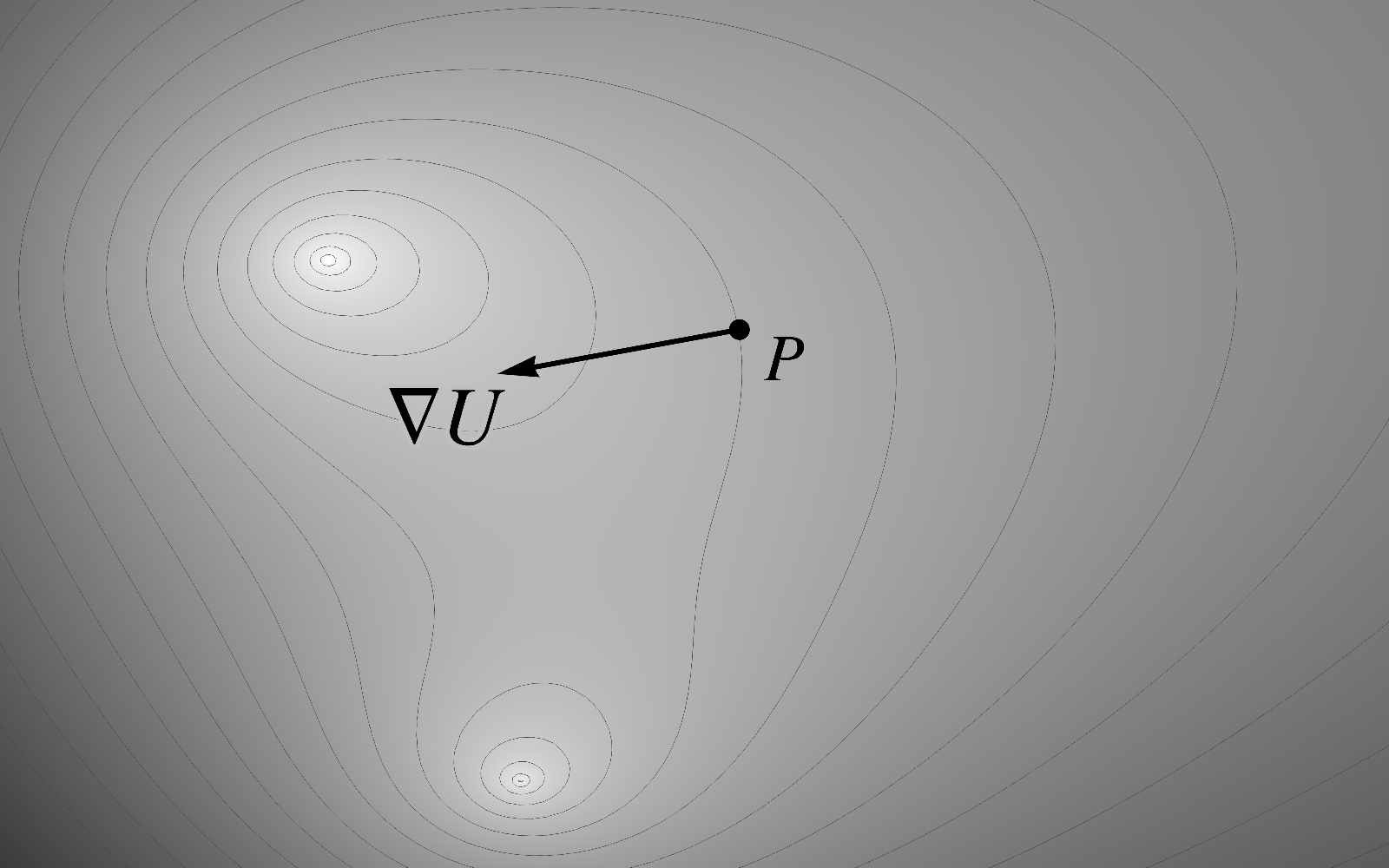 (4.76) The concept of the gradient applies
only to scalar fields since, as we discussed above, vectors cannot be compared in the same sense as
numbers, i.e. for two vectors, there is no rule for determining which one is "greater".
(4.76) The concept of the gradient applies
only to scalar fields since, as we discussed above, vectors cannot be compared in the same sense as
numbers, i.e. for two vectors, there is no rule for determining which one is "greater".
(4.76)Yet again, note the geometric nature of the newly introduced concept. For a given scalar field
, the gradient
can be evaluated, at least conceptually, by pure geometric means without a reference to a
coordinate system. Thus, our approach differs from that found in most textbooks where the gradient
is defined as a collection of partial derivatives. Later in this Chapter, we will begin the task of
reconciling the two approaches.
In the previous Section, we showed that the directional derivative of a scalar field at a point
in the
direction of the unit vector is given by
the dot product
where the vector is
independent of . You may
not be surprised to find out that equals the
gradient . Since is unit
length, the definition of the dot product tells us that
where is the angle between and . Since the
greatest value of is and occurs when , the greatest
possible value of is
and also occurs when , i.e. when the
unit vector points in
the direction of . Thus, the
vector indeed
represents the direction of the greatest increase in and,
furthermore, has the magnitude that equals the rate of the greatest increase. In other words, is the
gradient of , as we set
out to show. Having established this important connection, we can rewrite the directional
derivative formula
in the form
One of the insights offered by this formula is the fact that knowing the value of the gradient at a
given point is sufficient for determining the directional derivative in any direction . Furthermore,
the directional derivative of a scalar field is in any direction orthogonal to the gradient. Conversely,
if the directional derivative in a particular direction is , then the gradient is orthogonal to , provided
that the gradient is not zero. In particular, the gradient is orthogonal to the level sets of .
4.10Gradient examples
For the first example, again consider the function defined as the distance between the point
and an
arbitrary fixed point . It is
intuitively clear that the gradient of at a point is a unit
vector that points directly away from the point .  (4.80) It is left as an exercise to demonstrate this fact
analytically. Note that the gradient field is not defined at , where it
experiences a non-removable discontinuity.
(4.80) It is left as an exercise to demonstrate this fact
analytically. Note that the gradient field is not defined at , where it
experiences a non-removable discontinuity.
(4.80)For a second example, choose a fixed point along with a
ray emanating
from , and let
be the angle between the segment and the ray
, subject to
the condition that the angle varies between and and is measured in the
counterclockwise direction.  (4.81)
(4.81)It is intuitively clear that the gradient points in the counterclockwise direction orthogonal to
the segment and that its
magnitude is inversely proportional to the distance between and . To calculate
the precise magnitude of , note that a step of in the counterclockwise orthogonal direction
from results in
the change in that equals
.  (4.82) Thus, rate of change is given by the
limit
(4.82) Thus, rate of change is given by the
limit  (4.85) Once again, is discontinuous at .
(4.82) It is a matter of ordinary Calculus
to show that this limit equals , i.e.
The resulting gradient field is
illustrated in the following figure.
(4.85)4.11The coordinate representation of the gradient
In all likelihood, in your first encounter with the gradient, it was defined as the collection of
partial derivatives
with respect to Cartesian
coordinates . From this definition, it is then
demonstrated that the elements of represent the components of a vector
that points in the direction of the greatest increase of , while the
magnitude of that vector equals the corresponding greatest rate of increase. In other words, what
we have adopted as the definition of the gradient appears as a consequence in the
conventional approach.
Given that we now have two alternative definitions of the gradient, we must find a way to reconcile
them. Furthermore, we ought to generalize the coordinate space expression for the gradient to
general non-Cartesian coordinates. Looking ahead, the former task will be accomplished in Chapter
6 on coordinate systems while the latter will be
accomplished in Chapter 9 in which some of the most
fundamental coordinate-dependent objects will be introduced.
4.12Exercises
Exercise 4.1Show that for a circle of radius described by the vector equation of the curve , where is the central angle, the vector is tangential to the circle and has magnitude .
Exercise 4.2For the same equation of the curve , describe the vectors and in similar geometric terms.
4.12.1Properties of vector differentiation
Exercise 4.3Show that the derivative of vector-valued functions satisfies the sum rule
Exercise 4.4Show that for a constant number , the derivative of vector-valued functions satisfies the rule
Exercise 4.5Show that for a scalar function , the derivative of vector-valued functions satisfies the rule
Exercise 4.6Show that for a scalar function , the derivative of the composite vector-valued function satisfies the chain rule
Exercise 4.7Show that the derivative of vector-valued functions applied to the cross product satisfies the product rule
4.12.2Directional derivative and gradient exercises
Exercise 4.8Given two fixed points and in a three-dimensional space, let be the area of the triangle . Evaluate for pointing in the direction parallel to .
Exercise 4.9For the same function , evaluate for pointing in the direction orthogonal to and away from within the plane of the triangle .
Exercise 4.10For the same function , describe the gradient in geometric terms. Show that if the vectors , , and correspond to the points , , and , then points in the direction of the vector
and has the same magnitude as the vector .
Exercise 4.11Given two fixed points and , let . Describe the direction and the magnitude of , illustrated in the following figure, in geometric terms.  (4.89)
(4.89)4.12.3Motion of a material particle
Exercise 4.13In Section 4.5, we showed that the acceleration of a particle moving with constant speed is orthogonal to its trajectory. Show that the converse is also true: if the acceleration of a particle is orthogonal to its trajectory, then its speed is constant.
Exercise 4.14Consider a particle moving with constant speed. Show that
where is the acceleration vector.
Exercise 4.15Show that the trajectory of a particle moving in the plane with constant speed and non-zero acceleration of constant magnitude is a circle.
4.12.4Classical optimization problems
The minimization problems in the exercises below are intended to be solved by vector
differentiation and therefore require the following caveats commonly found in optimization problems
subject to differential analysis. First, all relevant curves must be sufficiently smooth. Second,
the minimum is meant in the local sense. Third, in problems related to curves, the optimal
point must lie in the interior of a curve.
Furthermore, most of the minimization problems below, when restated as maximization
problems, would yield the same criterion. However, in many common situation -- for instance, when
the relevant curves are unbounded -- a maximal solution does not exist while a minimal solution
exists under a broader range of conditions. This is one of the reasons why most problems are stated
as minimization problem.
Also note that in each of the problems, the criterion for a minimum can be stated in pure geometric
terms. In fact, you will observe that such a geometric interpretation will always be immediate and
obvious conclusions of your differential analysis. This is a significant strength of our approach
based on working with geometric vector quantities.
Finally, we should note that a geometric optimality criterion typically does not offer an algorithm
for constructing the optimal solution. Of course, this is typical of solving optimization
problems by differential analysis. Indeed, in ordinary Calculus, the extremal points of a function
are given by the equation -- however, Calculus does not tell us how to solve this
equation.
Exercise 4.16Given a point and a curve , suppose that a point that is closest to among all points on . Demonstrate that the location of is characterized by the fact that the segment is orthogonal to .  (4.91)
(4.91)Exercise 4.17Given two non-intersecting curves and , suppose that the segment represents the shortest distance between the two curves. Demonstrate that is orthogonal to each curve.  (4.92)
(4.92)Exercise 4.18Heron's problem: given two points and on one side of a straight line , suppose that the point on minimizes . Show that the location of is characterized by the "angle of incidence equals the angle of refraction" condition. Does your solution generalize from a straight line to a curve ?
Exercise 4.19The Torricelli point: given a triangle , where the largest angle is below , suppose that the point minimizes the sum of the distances from to the vertices. Demonstrate that is "equiangular" with respect to the vertices, i.e.