While in Chapter 4 curves played the secondary role
of illustrating vector-valued functions and their derivatives, in this Chapter, they will become
the central object of our analysis. However, we will save a full analytical description of curves
for a future book that will rely on the techniques developed in our present narrative. Instead, our
primary motivation is to continue exploring geometric concepts without the use of coordinate
systems, since in order to fully understand the power of coordinates, one must appreciate what is
possible in their absence.
That said, our present analysis will represent somewhat of a compromise with respect to the use of
coordinates. The ambient space will remain coordinate-free and we will therefore be working
directly with geometric vectors rather than their components. Meanwhile, the points on the curve
will be enumerated by a parameter , as was the case in the previous
Chapter for the curve associated a vector-valued function . There is no denying that the parameter amounts to a coordinate system on the
curve. Thus, while our analysis will remain mostly geometric and will, as a result, provide great
geometric clarity and insight, we will also begin to see some of the benefits of coordinate
systems.
At the same time, we will observe that the analytical methods developed in this Chapter are
insufficient for practical calculations, such as determining the curvature or the torsion of a
specific curve. Most practical calculations can only be reasonably accomplished when all
geometric objects are converted either into analytical expressions, which can be analyzed by means
of Algebra and Calculus, or into numerical data which can be analyzed by computational methods.
This is the role of coordinate systems.
In all of the following discussions, unless we are specifically discussing a planar curve,
you should imagine a curve in a three-dimensional space, such as the "spiraling funnel" in the
following figure.  (5.1) In the previous Chapter, we learned
that a curve is characterized by its unit tangent vector . We would
now like to add that a curve in a three-dimensional space is also characterized by a plane
orthogonal to known as
the normal plane.
(5.1) In the previous Chapter, we learned
that a curve is characterized by its unit tangent vector . We would
now like to add that a curve in a three-dimensional space is also characterized by a plane
orthogonal to known as
the normal plane.  (5.2) Thus, in three dimensions, there does not exist a unique
orthogonal direction, but rather a two-dimensional orthogonal space. Below, we will discover a
natural basis for this space.
(5.2) Thus, in three dimensions, there does not exist a unique
orthogonal direction, but rather a two-dimensional orthogonal space. Below, we will discover a
natural basis for this space.
(5.1)(5.2)5.1Arc-length parameterization
In Chapter 3, we discussed the possibility of
choosing a signed arc length parameterization on a curve. Denote by the corresponding vector equation of the
curve. In selecting an arc length parameterization, we have two arbitrary choices to make: the
location of the origin, i.e. the point where (which is distinct from the origin ), and the
orientation of the parameterization, i.e. the direction in which increases.  (5.3)
(5.3)
(5.3)An important intuitive characteristic of an arc-length parameterization is the regular spacing in
the sense of the distance along the curve between points corresponding to coordinates
separated by constant values. This is illustrated in the figure above. Note that while the figure
shows a planar curve, arc-length parameterization works perfectly well for curves in a
three-dimensional space and throughout the discussion, the reader should try to visualize
three-dimensional configurations.
As we established in Chapter 4 for general
vector equations of the curve, the derivative is tangential to the curve at each point.
However, in the special case of an arc length parameterization, satisfies the additional property that it is
unit length, i.e.
As a result, the vector is referred to as the unit tangent. We
will denote it by the symbol , i.e.
To see why is unit length, let us examine its
construction according to the limiting procedure described in Chapter 4. Consider two nearby points on the curve corresponding to the values of
the arc length and . For any value of , the distance along the curve between the two points
is, by definition, . When we consider a small , and zoom in on the section of the curve
between the two points, it will appear to be essentially straight. Therefore, the length of
the vector  (5.7) Had we chosen , the corresponding section of the curve would be
visually indistinguishable from , whose length would be approximately , i.e. times closer to compared to .
(5.7) Had we chosen , the corresponding section of the curve would be
visually indistinguishable from , whose length would be approximately , i.e. times closer to compared to .
will essentially equal , although, in actuality, it will be slightly
shorter. The following figure illustrates this insight at for , where the length of the vector is . We chose this value of because it is small enough to illustrate the
near-equality of and the length of , yet still large enough for us to see that the curve is not
actually straight.
(5.7)Since for small , the length of the vector is essentially , the length of the vector
is essentially and, in the limit as , it is
, i.e.
In other words,
as we set out to prove.
Thus, referring to as the unit tangent is justified. Note,
however, that at each point there are two unit tangents since the vector is also one. Nevertheless, having
arbitrarily selected one unit tangent out of the two available options, we can refer to it as
the unit tangent to indicate that the choice has already been made. Between these two
legitimate unit tangents, the derivative corresponds to the one that points in the
direction of increasing arc-length . In the future, we will observe this
interesting lack of uniqueness for other important geometric objects, including the unit normal
characterizing planar curves.
5.2The arc length integral
Let us now return to a curve parameterized by an arbitrary parameter . Our present goal is to demonstrate
that the integral  (5.11) Note that the integrand is simply the length of . However we prefer the expression since it
yields itself more readily to analytical manipulations.
(5.11) Note that the integrand is simply the length of . However we prefer the expression since it
yields itself more readily to analytical manipulations.
where ,
yields the arc length of the section of the curve between the points and corresponding
to and
.
(5.11)The integral
is our first example of a central
concept in Tensor Calculus -- that of an invariant. It is an invariant because it
yields the same value for any parameterization , provided that the limits of
integration correspond to the section of the curve between the points and and that
. The
fact that the above integral is an invariant means that its value is a characteristic of the
curve itself rather than that of a particular parameterization. And more often than not,
invariants, and especially those given by simple expressions, have a clear geometric meaning,
although that meaning may not always be apparent. In the particular case of the above integral, it
is the length of the curve between and
Before we prove this, we would like to point out two special parameterizations for which it
is intuitively so. First, if represents time and the curve,
therefore, corresponds to the trajectory of a material particle, then the vector represents the velocity of the particle,
while its magnitude represents
speed. Thus,
is an integral of speed over the
period of time from to
, and
thus represents the total distance traveled between those times. In other words, it is the length
of the curve between the points and .
Second, suppose that corresponds to arc length , and let the points and correspond to
the values and
, where
.  (5.12) The presumed length-of-curve integral for this
parameterization reads
(5.12) The presumed length-of-curve integral for this
parameterization reads
(5.12)
In the previous Section, we established that the length of is . Therefore,
and we have
By definition, the difference is
precisely to the length of the curve between the points and , as we set
out to show.
The arc length parameterization example can now serve as a starting point for the general
demonstration. Having shown that the integral
yields the length of the curve
between the points and for one
particular parameterization, we only need to prove that the above integral is independent of
parameterization. In other words, we must show that if the curve were alternatively parameterized
with the help of another variable , then
where the values and
also
correspond to the endpoints and , and . If
the values of both variables and increase in the same direction along
the curve, then must
correspond to and to
. Otherwise,
must
correspond to and to
.
An important remark regarding our notation is in order. Even though the symbols and use the same letter , they
represent different, albeit related, functions. For example, the symbol may represents both evaluated at and evaluated at . Naturally, those
are generally completely different vectors. Nevertheless, the two functions and represent the same geometric quantity, i.e.
the position vector , and are
therefore closely related enough to justify using the same letter. We can still easily distinguish
the two functions by the letter representing the argument, and doing so is a common and necessary
practice in Tensor Calculus that will be used extensively throughout our narrative.
Before we give the analytical argument that proves the identity
we would like to present a geometric
argument that will give you an intuitive feel for it. The essence of the argument is that if
the alternative parameterization is such that the vector is longer (or shorter) compared to , then the interval of integration shrinks (or
expands) correspondingly, leaving the value of the integral unchanged.
For an illustration, consider the two alternative parameterizations for the same curve in the
following figure.  (5.17) Notice that the relationship between
and is
(5.17) Notice that the relationship between
and is
(5.17) Whether we describe this change of
variables as stretching or shrinking the parameterization, let us show that the old tangent
vector is twice the length of the new tangent
vector .
Consider the point on the curve that corresponds to and . Next, identify
the points that correspond to increasing each parameter by . The point that corresponds to is located
roughly half way between the points corresponding to and . The point
corresponding to is located
roughly only a quarter of the way between the same two points. Thus, for the same value of
, the vector
is roughly twice as great as
and, in the limit as approaches zero, we find
Thus, the integrand in
is twice the integrand in
for corresponding values of and . However, the interval of integration
in the first integral is half that in the second integral for any given section of the
curve. Thus, the two effects balance each other and, as a result, the two integrals yield the same
value, as we set out to show.
Let us now turn to the formal proof of the fact that the integral
is independent of the
parameterization. Consider an alternative parameterization of the curve by the variable , where
corresponds to ,
corresponds to . Furthermore,
assume that , i.e.
the two parameterizations have the same orientation, meaning that the values of and increase in the same direction along
the curve. The proof for the case of opposite orientations is left as an exercise.
Suppose that and are related by the function , i.e.
where
For reasons that will become
apparent shortly, it is essential to use the same letter to denote both the variable itself and the function that
translates the values of to . Since the two parameterizations have
the same orientation, is monotonically increasing and therefore has
a positive derivative, i.e.
The functions and are related by substituting the function
into , i.e.
This identity makes it apparent why
it was necessary to reuse the letter for the function relating the
variables and . Had we denoted this function by a
different symbol, say , then, in the resulting expression , it would be unclear whether refers to
or . In the expression , on the other hand, the appearance of the
letter makes it clear that stands for
.
The equation
represents an identity in the
independent variable and can therefore be differentiated
with respect to . By the chain rule, we have
Substituting this result into the
integral
we find
where, in bringing from under the square root, we used the fact
that is positive. The resulting integral is
tailor-made for an application of the change-of-variables formula from ordinary Calculus, which
yields
as we set out to show.
5.2.1The rate of change of arc length
For a given parameterization , denote by the signed arc length with origin at
, i.e.
and assume that and have the same orientation. Then,
thanks to the result we have just established, can be expressed by the integral
By the Fundamental Theorem of
Calculus, the derivative is given by
Since is monotonically increasing, there also
exists an inverse function that expresses the parameter in terms of the signed arc length
. Its derivative is, of course, given by
It is a common occurrence when
working with inverse functions that the derivative of is expressed in terms of the values of the function rather than its independent variable . This may seem like an inconvenience, but it
will soon prove to our advantage.
If the arc length has the opposite orientation relative
to the parameter , then the function is given by the equation
while its derivative is given by
Then the derivative of the inverse
function is given by
This completes our discussion of the arc length integral and we will now turn our attention to
curvature.
5.3Curvature
Curvature is one of the central themes in Differential Geometry and we are about to take our
initial steps towards its analytical description. Our analysis will be based exclusively on
parameterizing the curve by its arc length .
5.3.1The curvature normal
Recall from earlier that the derivative of the position vector is a tangent vector of unit length known as
the unit tangent , i.e.
When we want to call attention to
the fact that is a
function of , we will use the symbol . Generally, the argument of a function may be
included for several purposes. First, when the represented quantity is being differentiated, the
argument indicates the independent variable with respect to which the differentiation is taking
place. Second, the argument can be used to distinguish between two different functions denoted by
the same later -- for example, and . Finally, it may be included simply to
emphasize the fact that the symbol denotes a function rather than an isolated object.
Let us now consider the derivative of the unit tangent vector and denote it by the symbol , i.e.
In Chapter 4, we demonstrated that the derivative of a vector of constant length is
orthogonal to it. Since is a vector of unit (and therefore constant)
length, its derivative , is
orthogonal to it, and since represents
the instantaneous direction of the curve, is said to
be orthogonal, or normal, to the curve.
Furthermore, since is of constant length, its derivative
measures solely the rate at which changes direction. What is the
underlying phenomenon responsible for changing its direction? Of course, it is what
we intuitively understand to be curvature. The greater the curvature, the greater the rate
of change in the direction of . The vector , therefore,
quantifies the concept of curvature. Thanks to its two signature properties -- being normal to the
curve and being characteristic of curvature -- the vector is known as
the curvature normal.  (5.39)
(5.39)Note that can be
expressed as the second derivative of the position vector , i.e.
Thus, curvature is a
second-derivative phenomenon.
Simply by imagining the way the unit tangent changes its direction as you travel along the curve,
you should be able to convince yourself that the curvature normal points in
the "inward" direction, i.e. the direction towards which the curve is bending. The figure
above shows for a
planar curve. The following figure shows the curvature normal for a
three-dimensional helical funnel.  (5.41) Note that the displayed length of is affected
by our angle of view.
(5.41) Note that the displayed length of is affected
by our angle of view.
(5.41)Another way to get a sense for the direction of is to
imagine yourself traveling by car with unit speed along the curve. The velocity of the car
corresponds to the tangent vector , while the acceleration corresponds to
the curvature normal . As you go around a bend, you will feel
yourself being pulled in the outward direction by the apparent centrifugal force. This is so
because your actual acceleration, i.e. , points
inward. Note that this effect is independent of the direction in which the car is travelling and we
will now take a closer look at this phenomenon.
5.3.2A note on signs
Unlike the unit normal , whose
direction depends on the orientation of the parameterization, the curvature normal is
independent of it. This can be seen in a number of insightful ways. The first way is to consider
the finite difference  (5.43) Note that in both scenarios, the tangent vector turns inward
as increases and therefore the vector also points in the inward direction. Thus, in the limit as
, the before also points inward.
(5.43) Note that in both scenarios, the tangent vector turns inward
as increases and therefore the vector also points in the inward direction. Thus, in the limit as
, the before also points inward.
for two parameterizations with
opposite orientations, as illustrated in the following figure.
(5.43)A related intuitive way to justify the independence of from the
orientation of the parameterization is to interpret the parameter as time and to imagine a hammer thrower in
the act of spinning the "hammer", i.e. a metal ball attached by a wire to a handle. Prior to its
release, the ball is kept in circular motion by the string's tension. The acceleration of the ball
points in the direction of the tension force, i.e. inward, which is the case regardless
of the direction in which the hammer is is spun.  (5.44)
(5.44)Finally, the independence of from the
orientation of the parameterization can be demonstrated by a formal analytical calculation. Let
be an
arc length parameterization that has the opposite orientation with respect to . Assuming and share
the same origin, we have
If we treat as a function of , then
Consider the two functions and that represent the position
vector with respect to and . Then
can be expressed as a
composition of and , i.e.
Differentiating the above identity
with respect to , we
find
In other words,
at corresponding values of and , which
confirms that the unit tangents associated with each parameterization point in the opposite
directions.
Next, convert the above equation into an identity with respect to , i.e.
Differentiating once again with
respect to , we
find
In summary,
or
as we set out to show. In general,
odd-ordered derivatives of and are opposite of each other while even-ordered
derivatives are identical.
5.3.3The absolute curvature and the principal normal
The magnitude of is known as
the absolute curvature and is denoted by , i.e.
The term absolute refers to
the fact that is always
nonnegative. However, absolute is often omitted and is referred
to simply as curvature, although we have to exercise care since we will also work with the
related concept of signed curvature for planar curves which may also be casually
referred to as curvature, but may differ in sign from .
The unit vector that points
in the same direction as is called
the principal normal. Thus, the curvature normal is the
product of the absolute curvature and the
principal normal , i.e.
The principal normal field for a planar curve is illustrated in the following figure.  (5.56) Note, importantly, that the principal normal is undefined at
points of inflection where it undergoes a nonremovable discontinuity. The following figure
illustrates the principal normal for a
three-dimensional helical funnel.
(5.56) Note, importantly, that the principal normal is undefined at
points of inflection where it undergoes a nonremovable discontinuity. The following figure
illustrates the principal normal for a
three-dimensional helical funnel.  (5.57)
(5.56)(5.57)By definition, the principal normal is found in
the normal plane, and thus singles out a particular direction in the two-dimensional normal space.
 (5.58) It can therefore act as an element in
a natural basis for the normal plane. Later in this Chapter, we will supplement with a vector , orthogonal to both and , that will
complete the basis.
(5.58) It can therefore act as an element in
a natural basis for the normal plane. Later in this Chapter, we will supplement with a vector , orthogonal to both and , that will
complete the basis.
(5.58)5.3.4Planar curves and signed curvature
Let us briefly turn our attention to planar curves. Whereas for curves in three dimensions we find
a two-dimensional normal space, planar curves are characterized by a one-dimensional normal space.
In other words, the normal direction is unique, and this is a common characteristic of
hypersurfaces, i.e. geometric shapes whose dimension trails that of the surrounding space by
, such as planar curves and two-dimensional surfaces in a
three-dimensional space.  (5.59)
(5.59)Thus, we know the direction (to within sign) of the principal normal as soon as
we have calculated the tangent . In fact,
for hypersurfaces, it is common to establish the unique normal direction prior to the analysis of
curvature. This is usually accomplished by arbitrarily selecting one of two opposite normal
directions. The unit vector pointing in
the selected direction is referred to as the unit normal. As in the case of the unit
tangent, the article the indicates that the choice has already been made. The freedom to
choose one of the two opposite unit normals is referred to as the choice of normal. In
practice, it is common to choose a consistent normal direction so that the resulting normal
field is globally continuous. The following figure shows two alternative choices of normal that
result in continuous normal fields.  (5.60)
(5.60)Recall that unlike the unit normal , the
curvature normal is uniquely
determined by the shape of the curve. Since also points
in the normal direction, it is colinear with the unit normal . Thus,
is a scalar
multiple of , i.e.
The number is known as the signed curvature. It
is a special case of the beautiful concept of mean curvature that characterizes general
hypersurfaces. Mean curvature will be described in a future book and, from the moment of its
introduction, will play a crucial role in most of our subsequent explorations.
Crucially, the sign of depends on the choice of normal. It equals
the magnitude of when the
latter points in the same direction as and
minus the magnitude of otherwise.
This fact can be expressed by the equation
The same equation in terms of the
unit tangent reads
Much like the absolute curvature , the signed
curvature is also often referred to simply as
curvature, making the term curvature ambiguous for planar curves. To catalog the
relationship between and , recall that  (5.65)
where is the
principal normal. Note that both and
equal the curvature normal , i.e.
Thus, when
(and ) point in
the same direction as , and otherwise. The relationship among , , , and is
illustrated in the following figure.
(5.65)To reiterate, our entire discussion of signed curvature has been predicated on the choice of normal
having been
arbitrarily made. Had we made the opposite choice of normal, would have had the opposite value. Thus, the
phrase signed curvature with respect to the normal is often
used to describe . Meanwhile, the product is independent of the choice of normal since both and change sign
when the choice of normal is reversed.
Finally, note that the ambiguity in the choice of normal can be removed by coordinating the unit
normal with the unit tangent. For example, we could agree to always choose so that the
set is positively oriented. In other words, is obtained
from by a
counterclockwise rotation. There is an advantage to this approach: choosing in this way
enables us to determine which way the curve is bending simply by examining the sign of . Namely, the curve is bending
counterclockwise when and clockwise when .
5.4Torsion
Curvature characterizes the rate at which a curve deviates from being straight.
Torsion characterizes the rate which a curve deviates from being planar.
5.4.1The osculating plane
The plane spanned by the tangent and the principal normal directions and is known as
the osculating plane. The verb to osculate comes from the Latin word
osculum which means to kiss. While the tangent line captures the instantaneous
direction of the curve, the osculating plane captures its instantaneous plane of
"motion" as it accommodates both the "velocity" and the
"acceleration" .
5.4.2The binormal
The orthonormal vectors and form a
basis for the osculating plane. As a set, and are one
vector short of spanning the entire three-dimensional space. This shortfall can be remedied by
adding a unit vector that is orthogonal to both and . Between
the two vectors that satisfy this condition, choose so that the set is
positively oriented. (The concept of the orientation of a set of vectors was discussed in Chapter
3.) We wish the vectors , , and had arisen in alphabetical order, but alas! Fortunately, the
set , which features the same vectors in alphabetical
order, has the same orientation as .  (5.66)
(5.66)The resulting vector is known as the binormal vector or, simply, the
binormal. The binormal can be expressed in terms of the unit tangent and the
principal normal with the
help of the cross product, i.e.
Collectively, the vectors , , and are known as a Frenet or Frenet-Serret frame,
but can also be referred to as a local frame. The principal normal and the
binormal form a basis in the normal space.
5.4.3The definition of torsion
For the sake of brevity, we will now begin to drop the argument from most symbols and denote the derivatives
by the subscript rather than a prime, i.e.
Recall that the derivative of the position vector with
respect to yields the unit tangent . The
derivative of , in turn,
leads to the concepts of absolute curvature and principal
normal . As we
might expect, the derivative of gives rise
to yet another differential characteristic of the curve.
Let us represent as a
linear combination of , , and , i.e.
and determine each component in
turn.
The component of with
respect to is given by
the dot product  (5.78) Therefore, the projection of onto
equals the
projection of onto
, which is what the above equation is telling us.
(5.78) Therefore, the projection of onto
equals the
projection of onto
, which is what the above equation is telling us.
By the product rule,
Since is
orthogonal to , the first
term vanishes and we have
Recall that is, by
definition, the curvature normal ,
i.e.
and, therefore,
Finally, since is unit
length, its dot product with itself equals and therefore
This identity makes a great deal of
intuitive sense, especially for a planar curve. After all, the unit vectors and are locked
in an orthogonal relationship. As a result, whatever the rate at which is rotating
-- which, of course, is proportional to -- is rotating
at the same rate, as illustrated in the following figure.
(5.78)The coefficient of with
respect to , given by
the dot product
is easily seen to be zero, i.e.
since is of constant length and therefore is
orthogonal to .
Finally, let us turn our attention to the final coefficient of with
respect to given by
Unlike the components of with
respect to and , its
component with respect to the binormal cannot be expressed in terms of the quantities that have
already been introduced. After all, a curve in a three-dimensional space cannot be described by its
curvature alone. The absolute curvature characterizes the shape of the curve within the osculating
plane spanned by and . However,
the derivative is not
necessarily contained in the osculating plane. Therefore, its component with respect to the binormal , which is orthogonal to and , captures
the rate at which the curve escapes the osculating plane and corresponds to a new geometric
quantity.
The component of with
respect to the binormal is known as the torsion , i.e.
In particular, the full expansion of
with
respect to , , and reads
Unlike the absolute curvature , the torsion
can be both
positive and negative, as will be demonstrated in the upcoming example involving two helices of
opposite orientations. Also note that the value of torsion does not depend on the orientation of
the parameter . Indeed, recall when the parameterization is
reversed, changes its
direction and remains
unchanged. Meanwhile , being the cross product of and , also
changes its direction. It is left as an exercise to show that the derivative also
changes its direction. Thus, since both and
change their directions, their dot product, i.e. the torsion
, remains
unchanged.
5.4.4An illustration of torsion with two oppositely-oriented helices
The shape of a spring is known as a helix. A helix is great for illustrating the interplay
between curvature and torsion as it is characterized by constant values of both quantities. Helical
shapes commonly encountered in everyday life include the aforementioned springs, threads on bolts,
spiral staircases, and (with apologies to anyone reading these lines before 1940 or after 2025)
slinkies.
A helix can have one of two orientations. Suppose that the axis of a helix is aligned with a ray
pointing in the direction arbitrarily labeled as up. Then a right-handed helix twists
in the counterclockwise direction as it goes up, while a left-handed helix twists in the
clockwise direction. Threads on most bolts and screws are right-handed and are sometimes described
by the mnemonic righty-tighty. Importantly, rigidly rotating a helix upside down does not
change its orientation. In other words, one of the helices cannot be transformed into the other by
turning it upside down. Instead, it will remain equivalent to itself. We know this from our
everyday experience and will confirm it analytically by calculating the torsion of each helix. 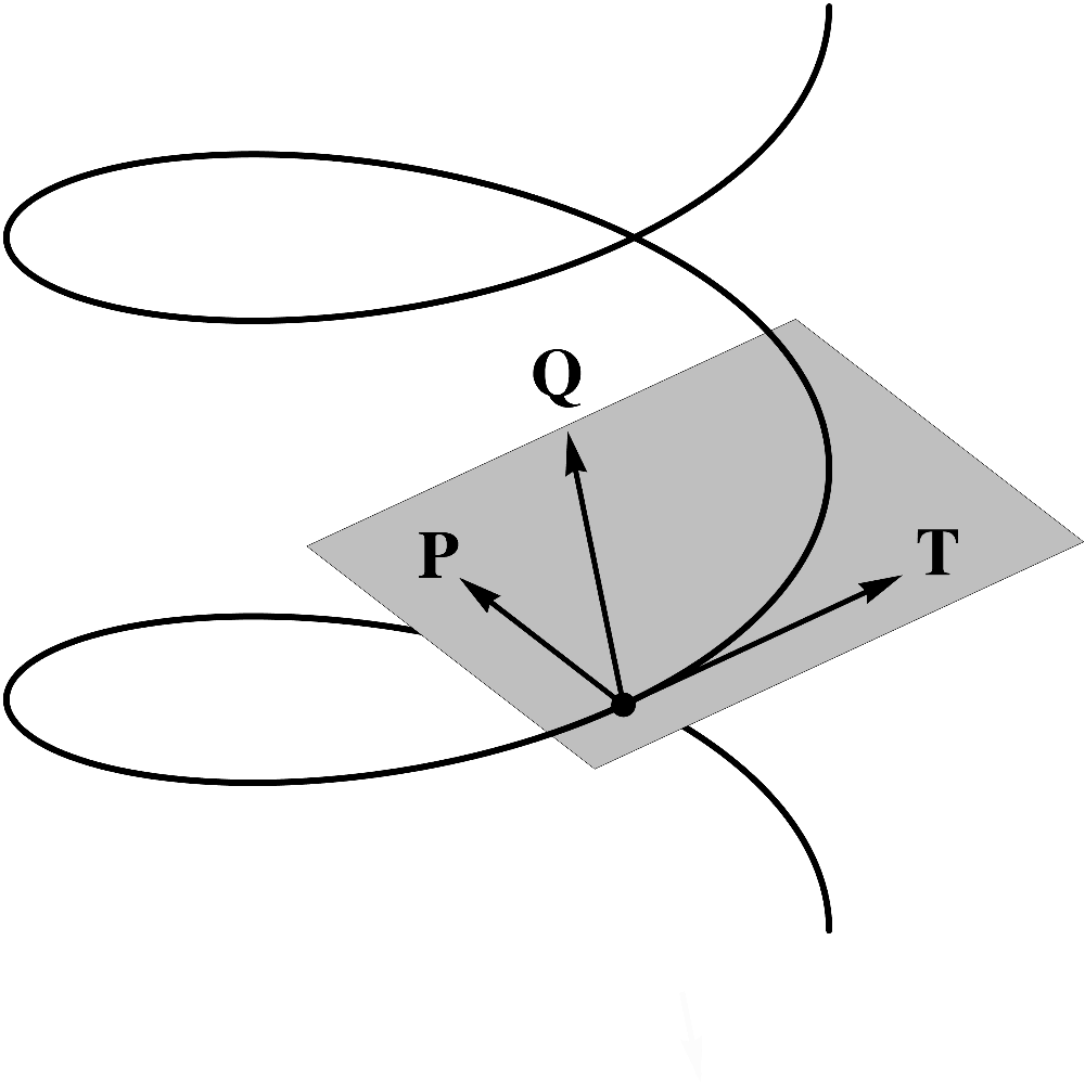
 (5.84)
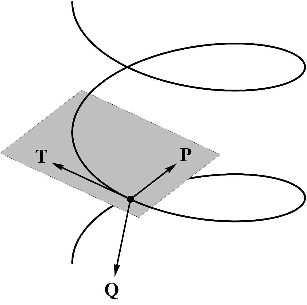
(5.84)In the above figure, the helix on the left is right-handed while the one on the right is
left-handed. As we discussed above, the orientation of the parameterization does not affect the
value of torsion. Therefore, assume that the parameter increases in the upward direction for both
helices. Then, for both shapes, the unit tangent points
slightly up, while the principal normal points
directly towards the axis in the strictly horizontal plane. (This property of is
intuitively clear from the fact that the upward "motion" is uniform and, thus, the "acceleration"
has no vertical component.) By the right-hand rule, the binormal points mostly up for the right-handed helix and mostly down
for the left-handed helix.
Now, let us get a sense for the derivative of the
principal normal . Since
remains in
the horizontal plane for all values of , its derivative is
also found in that plane. Within that plane, rotates in
the counterclockwise direction for the right-handed helix and in the clockwise direction for the
left-handed helix. Furthermore, we know that is
also contained in the plane spanned by and . Thus, let us examine how it is arranged in that plane
relative to and . The following figure shows the plane spanned by and for both helices. Since rotates in
the counterclockwise direction for the right-handed helix, points
to the left. Correspondingly, points
to the right for the left-handed helix. 
 (5.85) Observe that
for the right-handed helix, the component with
respect to , i.e. the torsion , is positive.
Meanwhile, for the left-handed helix, it is negative.
(5.85) Observe that
for the right-handed helix, the component with
respect to , i.e. the torsion , is positive.
Meanwhile, for the left-handed helix, it is negative.
(5.85)This also proves that one type of helix cannot be transformed into the other by a rigid rotation.
Indeed, since torsion depends only on the shape of the curve, it cannot be changed by a rigid
rotation. Therefore, the torsion on the helix, say, on the left will remain positive if that helix
were rotated upside down. Therefore, the upside-down version of the helix on the left is still
fundamentally distinct from the helix on the right whose torsion is negative.
Finally, this is an opportune moment to reiterate an important point that we made at the beginning
of the Chapter. Namely, despite the great geometric insight that we have been able to achieve, our
geometric approach does not enable us to calculate either the absolute curvature or the
torsion for a specific
curve -- at least, not easily. After all, the helix is the simplest conceivable three-dimensional
curve with nonvanishing curvature and torsion and we do not yet have an effective tool for
determining the numerical value of or . This
observation makes clear the need for a more robust analytical network. This will be achieved by the
introduction of a coordinate system in the ambient space and the subsequent development of a tensor
framework, which will enable us to work with the components of vectors rather than the
vectors themselves since the components of vectors can be analyzed by the powerful methods of
Calculus or -- when a reasonable analytical approach is not feasible -- numerical methods.
5.5The Frenet equations
5.5.1The derivative of the binormal
It is only natural to wonder whether the derivative of the
binormal produces yet another differential characteristic of the curve
that would join the ranks of curvature and torsion. To this end, let us decompose with
respect to the local frame , i.e.
Since is unit length, is
orthogonal to and therefore
The components and of with
respect to and are given
by the dot products
In both cases, an application of the
product rule will transfer the derivative from onto
the other vector. For , we have
Since is orthogonal to , the first
term vanishes and thus
Recall that and
therefore
Finally, since is orthogonal to , we
conclude that vanishes, i.e.
For the component of with
respect to the principal normal , the same
approach yields the following chain of identities.
In summary, the complete decomposition of with
respect to , , and reads
Thus, the analysis of has
not lead to a new differential characteristic of a curve. It would therefore appear that the
curvature and the torsion capture all of the available information about the local behavior of a
curve. In fact, as we demonstrate below, if the functions and are stated a priori, they are
sufficient to reconstruct the shape of the curve in a three-dimensional space.
5.5.2The statement of the Frenet equations
Let us combine the decompositions of , , and
in
terms of , , and into a single set, i.e.
Collectively, these equations are known as the Frenet formulas or the Frenet-Serret
formulas. In matrix form, the equations read
and it becomes apparent how these
formulas might generalize to higher-dimensional spaces. Indeed, this generalization will be
accomplished in Chapter 20 on Riemannian spaces.
5.5.3The intrinsic equation of a curve
One of the insights provided by the Frenet equations is that the shape of a curve is fully
specified by the curvature and torsion as functions of arc length. Suppose that the functions and are given, along with the ambient location of
one point on the curve, say, at , and
the curve's orientation at that point. In other words, let the values , , , and therefore , be
known. Then the entire curve can be reconstructed by solving the system of ordinary differential
equations
subject to the initial conditions
Once is
calculated, can be
reconstructed by solving the equation
subject to the initial condition
Of course, could have
been included among the unknowns, resulting in a system with equations and unknowns, but that would have diminished the elegance of
the system and its closure under the functions , , and .
Because and , along with the initial conditions, are
sufficient to describe the shape, the location, and the orientation of the curve, these functions
are known as the intrinsic, or natural, equations of the curve. In the absence
of initial conditions, the functions and are still sufficient to determine the shape
of the curve.
5.5.4The Frenet equations for a general parameterization
The foregoing analysis took fundamental advantage of the special parameterization of the curve with
the help of the arc length . In practice, however, an arc-length
parameterization is difficult to achieve for specific curves. Meanwhile, a different
parameterization may be readily available. It is of interest, then, to adapt the above analysis to
a parameterization with an arbitrary variable . Since the only parameter-dependent
operation in our analysis is the derivative, all we need to do is express in terms of .
Suppose that a quantity , scalar or
vector, is defined on the curve. Consider it simultaneously as functions and of and . The functions and are related by the identity
where is dependence of the variable on the arc length . Then, by the chain rule, we find
Isolating the operators and , we have
Recall that the derivative is given by the equation
This is where the fact that the
derivative is naturally expressed as a function of rather than , is advantageous since it enables us to
express explicitly in terms of and , i.e.
With the help of this equation, can
now rewrite the Frenet equations for a curve subject to an arbitrary parameterization. Letting
we have
This form greatly increases the applicability of the Frenet formulas. Nevertheless, it remains fair
to say that all equations presented so far have mostly theoretical applications due to the use of
geometric vectors which have limited analytical capabilities. In order to facilitate practical
calculations, it is necessary to refer the ambient space to a coordinate system in order to enable
us to work with the components of vectors rather than the vectors themselves. This is the task that
we will begin to undertake in the next Chapter.
5.6Exercises
Exercise 5.1What is the geometric interpretation of the integral
Conclude that for a closed curve, i.e. ,
Exercise 5.2Similarly, what is the geometric interpretation of the integral
For this integral, too, conclude that for a closed curve,
Note that for the conclusions of this exercise to hold, the curve must be free of kinks, i.e. must be continous.
Exercise 5.3Complete the proof of the fact that
is independent of parameterization by analyzing an alternative parameterization whose orientation is opposite that of .
Exercise 5.4Show that the absolute curvature of a circle of radius is given by
Exercise 5.5Show that the signed curvature of a circle of radius with respect to the outward normal is given by
Exercise 5.6Explain why the derivative of the principal normal changes direction when the orientation of the parameterization is reversed.
Exercise 5.7In Section 5.5.1, justify each step in the chain of identities leading to the coefficient .
Exercise 5.8Derive the third Frenet equation
by differentiating the identity
Exercise 5.9Show that the Frenet equations for a planar curve read
Exercise 5.10Solve the planar Frenet equations for constant absolute curvature to show the resulting curve is a circle of radius .