Mathematics is a tool for finding order within the chaotic reality. Oftentimes, however,
mathematical methods create their own chaos, which impedes their progress. This is the case for the
method of coordinates, which is deservedly considered one of the greatest breakthroughs in
the history of mathematical thought. Tensor Calculus represents an analytical framework that
harnesses the power of coordinates while mitigating the unwanted artifacts that otherwise accompany
them. Thus, Tensor Calculus can be described as the art of using coordinate systems to gain deep
insights into the nature of space and time and therefore a wide range of physical phenomena.
But this is not the main reason why you should read this book. You should read this book because
Tensor Calculus is a breathtakingly beautiful subject that will help you organize your knowledge,
and thus improve your understanding of fundamental Applied Mathematics -- in particular,
multivariable Calculus and its interplay with Linear Algebra. Tensor Calculus will improve your
ability to think geometrically, algebraically, and algorithmically at the same time. And, perhaps
most importantly, I hope that you will take inspiration from this subject on how to choose a
starting point in your investigations and proceed confidently from it.
1.1Tensor Calculus as a junction of Algebra and Geometry
Tensor Calculus is many things at once, but the original impetus behind its invention was the
development of an analytical framework for preserving the geometric meaning in calculations
involving coordinate systems. The resulting framework succeeds in achieving this goal beyond
expectations. Tensor Calculus has proven to be a powerful tool for scientific investigations and
has provided a path to many important discoveries in Mathematics and Physics.
The invention of coordinate systems in the seventeenth century ushered in the era of close
interplay between Algebra and Geometry. The often quoted pronouncement by Lagrange perfectly
captures the importance of that interaction: As long as algebra and geometry proceeded along
separate paths, their advance was slow and their applications limited. But when these sciences
joined forces, they drew from each other fresh vitality and thenceforward marched on at a rapid
pace toward perfection.
Over the next three centuries, the cross-pollination of geometric and algebraic ideas led to the
development of a number of analytical subjects built upon ideas from geometry. A central place
among those subjects is occupied by Linear Algebra. While the modern applications of Linear Algebra
go far beyond geometric problems, its origins are fundamentally geometric. Many of its applications
that seemingly have little or nothing to do with geometry, such as deep learning, rely on essential
geometric notions of transformation and distance.
In its relationship to Geometry, Tensor Calculus may be thought of as an extension of Linear
Algebra. While Linear Algebra studies straight objects in straight spaces, Tensor Calculus studies
curved objects in curved spaces. Straight objects can be studied with Algebra. The presence of
curvature necessitates the use of Calculus. That is why Linear Algebra is an algebra while
Tensor Calculus is a calculus.
1.2Tensor Calculus and coordinate systems
Coordinate systems unlock the power of analytical methods in geometric applications. However, the
immense robustness of the coordinate approach also creates a tendency to use it with unnuanced
bluntness. In some circumstances, a certain lack of finesse does not necessarily get us into
trouble. Relatively simple calculations allow us to get away with it, as evidenced by many examples
in Calculus and Physics textbooks that involve solving a special problem with the help of a special
coordinate system. This creates the profoundly wrong impression that the mathematical description
of the natural world can be constructed with such calculations. In actuality, while special
coordinate systems are indeed well-suited for a wide range of tasks, some of the most imaginative,
profound, and intellectually satisfying mathematical ideas lie well beyond their reach.
An even more fundamental problem lies not in which coordinate systems are used but
how coordinate systems are used. Generally speaking, a problem solved by geometric means
requires an individual approach and at least some degree of ingenuity. Analytical methods, on the
other hand, are more universal and robust. As a result, there is a tendency to completely
replace the geometric problem with an analytical one. However, in doing so, we risk throwing out
the baby with the bathwater. When analytical calculations are disengaged from the geometry, it
usually becomes impossible to reconstruct the geometric meaning of the eventual analytical answer.
This point can be illustrated by Euler's analysis of minimal surfaces, i.e. surfaces of
least area, found in his 1744 treatise Methodus inveniendi lineas curvas maximi minimive
proprietate gaudentes, sive solutio problematis isoperimetrici lattissimo sensu accepti, which
can be translated as A method for finding curves with properties of maximum or minimum, or
solution of isoperimetric problems in the broadest possible sense. In this work, considered by
many to be one of the most beautiful mathematical works ever written, Euler laid a foundation for a
new branch of Mathematics that later became known as the Calculus of Variations.
As an illustration of his new method, Euler found a minimal surface of revolution which he showed
to be catenoid, i.e. the surface of revolution generated by a catenary. 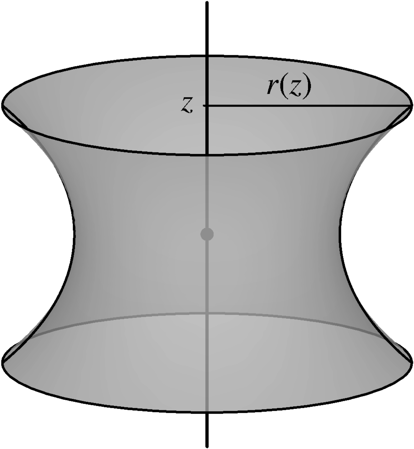 (1.1) Operating in cylindrical coordinates, Euler described the
unknown minimal surface by the function . He showed that satisfies the differential equation
(1.1) Operating in cylindrical coordinates, Euler described the
unknown minimal surface by the function . He showed that satisfies the differential equation
(1.1) which he then solved to reveal that
and thus describes a catenary. This
was the first instance of an explicit equation for a minimal surface. Despite this singular
breakthrough, Euler's approach did not reveal to him the geometric meaning of the differential
equation -- namely, that a minimal surface is characterized by zero mean curvature . This
was realized only half a century later by the French mathematician Jean Baptiste Meusnier. This
example teaches us that special care must be taken to preserve the connection between the analysis
and the geometry.
Another unavoidable consequence of the loss of geometric meaning is the rapid growth in the
complexity of the analytical expressions. Consider the expression for the mean curvature
of a surface given by the equation
in Cartesian coordinates. An expression of
this complexity would be an appropriate destination of an analytical investigation, but certainly
not an acceptable point of departure. Countless analyses never see the light of day as a result of
the mathematician retreating in the face of overwhelming complexity.
The underlying reason for the loss of the geometric insight lies not in choosing the wrong
coordinate system for the task, but in committing to a specific coordinate system too early
in one's analysis. The use of any specific coordinate system invariably obscures the true
meaning of the expressions by introducing the artifacts of that system's particular
characteristics.
1.3Tensor Calculus in a nutshell
Tensor Calculus solves this problem by restricting its attention to algorithms that work
simultaneously in all coordinate systems. This restriction is severe, but it ensures
no specific coordinate system has the opportunity to let its artifacts obscure the geometric
meaning. As a result, Tensor Calculus offers the best of both worlds: it produces universal
analytical expressions with a clear geometric meaning that can be evaluated in any
coordinate system according to a prescribed algorithm. Thus, the framework keeps Geometry and
Algebra joined at the hip by embracing the use of coordinate systems while organizing the
calculations in such a way that the geometric meaning (or something close to it) can be readily
restored for any intermediate object. In order to achieve this result, Tensor Calculus relies on
several elements.
First is the way coordinate systems are utilized. All coordinate systems used in the course of
constructing the framework are completely general, i.e. never specified in a concrete way and never
presumed to have any special features beyond some essential differentiability characteristics.
Coordinates will be denoted by symbols with superscripts, e.g. ,
, and
or,
collectively, . The
use of superscripts will be carefully explained starting with Chapter 7 on the tensor notation and finally culminating in Chapter 14 on the tensor property.
Second is the fundamental concepts of a variant and a tensor . A variant is an
object that is constructed by a specific algorithm that references the coordinates in the same way
in all coordinate systems. For example, for a temperature field in the domain
, the collection of partial derivatives with respect to
the coordinates, i.e.
or, collectively,
is a variant. It is a variant
because the algorithm that reads differentiate with
respect to each of the coordinates is the same in all coordinate systems. By the same token,
the collection of the second-order partial derivatives
is also a variant.
A variant is characterized by its order, i.e. the number of indices required to enumerate
its elements. Since, at any given physical point, the temperature field is a single
number, it does not require any enumeration and is therefore considered to be a variant of order
zero. The collection of the partial derivatives is a
variant of order one, while the collection of second-order derivatives
is a variant of order two.
Variants are subject to a series of operations that include addition, multiplication, covariant
differentiation, and contraction. Addition applies to variants of the same order and produces
another variant of the same order. Multiplication applies to variants of arbitrary orders and
produces a variant of the combined order. Covariant differentiation increases the order by one.
Contraction decreases the order by two.
Crucially, the values of a variant change from one coordinate system to another -- thus the name
variant. In the example above, the temperature field itself does
not change from one coordinate system to another. That makes it a special kind of variant known as
an invariant. The values of and
,
on the other hand, certainly vary from one coordinate system to another. The relationship between
the values of a variant in different coordinate systems is known as the transformation rule.
This brings us to tensors. A tensor is a variant of a special kind that transforms from one
coordinate system to another by a particular rule known as the tensor transformation rule.
Crucially, there are two opposite flavors of tensor transformations: covariant and
contravariant. The two transformation rules oppose each other in the sense of the matrix
inverse. This inverse relationship is the key to the eventual elimination of the nongeometric
artifacts of coordinate systems. When the covariant mode encounters a contravariant mode and the
accompanying transformation matrix meets its inverse, the operation of contraction forces the two
matrices to multiply and therefore cancel each other's influences, thus bringing the combination a
step closer to invariance.
Tensors possess three properties that enable them to faithfully preserve the geometry of the
initial problem. First, the components of a geometric vector form a tensor. Second, tensors are
closed under addition, multiplication, covariant differentiation, and contraction. Third, when a
tensor is reduced to order zero by contraction or a series of contractions, the resulting value is
the same in all coordinate systems. Checkmate.
A variant of order zero, i.e. a single quantity, that has the same value in all coordinate systems
is known as an invariant. Since the value of an invariant does not depend on the choice of
coordinates, it must have an independent geometric significance. Experience shows that for simpler
invariants, we are able to find a way to calculate the same value by a geometric construction.
The overall logic of the tensor framework is, therefore, not surprising since it follows that of
component spaces in Linear Algebra. Component space analysis in Linear Algebra starts with
decomposition, i.e. the translation of "real life" objects into their components with respect to a
basis. The bulk of the analysis is subsequently conducted in terms of the components, thanks to the
analytical robustness of the component space which has recently been boosted further by the
relatively newly-acquired ability to delegate complex computational tasks to electronic devices. In
the final step, the results of the component analysis are reinterpreted in the real world by
recombining their components with the original basis.
In Tensor Calculus, the first step is the same: decomposition with respect to a basis. The fact
that the components of a vector form a tensor ensures that the analysis starts in the tensor space.
The bulk of the analysis then proceeds in the component space. We must therefore develop a
framework that ensures that all intermediate objects are tensors. Much of our energies will be
directed towards this task. The main difficulty lies with differentiation, as it does not preserve
the tensor property, and the main breakthrough is achieved with the introduction of the
covariant derivative. The covariant derivative is an extension of the ordinary derivative
that preserves the tensor property. It therefore replaces the ordinary derivative in all aspects of
the analysis. Having thus assured that the tensor property of objects is preserved throughout the
analysis, contraction produces an invariant in the final step, thus bringing us back to "real
life".
In summary, Tensor Calculus combines the best of the geometric and algebraic worlds. It enables us
to leverage the unmatched utility of coordinate systems in a way that faithfully preserves the
geometric meaning of the objects under investigation.