In this Chapter, we will describe additional geometric concepts available in a Euclidean space that
will play an important role in our approach to Tensor Calculus. Even if some of these concepts are
already familiar to you, you may find our particular approach to be different from what is found in
most contemporary texts. Namely, we will continue to introduce concepts in a pure geometric context
without any reference to coordinates. Thus, Euclidean spaces will continue to serve as absolute
references for our analytical investigations.
3.1The orientation of a set of vectors
In a Euclidean space, a basis -- i.e. an ordered set of linearly independent vectors whose number
matches the dimension of the space -- can be described as either positively or negatively
oriented. The concept of orientation works in each natural Euclidean dimension, i.e. one, two,
and three, and is critical for several important objects that we will introduce in the future,
including the Levi-Civita symbol in
Chapter 17 and the curl operator in Chapter
18.
Interestingly, the concept of orientation can be almost completely sidestepped, as was done in the
predecessor to this book, Introduction to Tensor Analysis and the Calculus of Moving
Surfaces, as well as numerous other texts on Tensor Calculus. However, this concept admits such
an elegant geometric approach and thus fits so perfectly into our present narrative, that there is
much to be gained by discussing it in significant detail.
3.1.1In three dimensions
Let us begin our discussion in three dimensions where the concept of orientation is at its richest.
Consider an ordered set of three linearly independent vectors , , and and let be the plane
spanned by and .  (3.1) The plane splits the
three-dimensional space into two half-spaces. Since the vectors , , and are linearly independent, and thus
the vector cannot lie in the plane , it is found
either in one or the other half-space.
(3.1) The plane splits the
three-dimensional space into two half-spaces. Since the vectors , , and are linearly independent, and thus
the vector cannot lie in the plane , it is found
either in one or the other half-space. 
 (3.2)
(3.2)
(3.1) (3.2)Within , the vector
can be
rotated towards in one of two directions. In one
direction, the rotation is less than and
in the other -- greater than . If
is found in the half-space from which
the shorter rotation appears counterclockwise then the ordered set is said to be positively
oriented. Otherwise, it is negatively oriented. In the figure above, the set of vectors
on the left is positively oriented, while the one on the right is negatively oriented.
The same criterion can also be expressed in the form of the right-hand rule: if you curl the
fingers of your right hand in the direction of the shorter rotation from to and the thumb of that hand points
towards the half-space containing , then the set is positively
oriented. Note that the right-hand rule relies on the ability to choose the correct hand for
the task. Mistakenly choosing the left hand would, naturally, lead to the wrong conclusion. Thus,
the right-hand rule relies on the preexisting convention of which hand is right. If humanity
lost its collective sense of right, there may not exist a reliable way of restoring it back
to its present meaning.
The same can be said of the notion of counterclockwise rotation in our initial formulation
of the criterion. It therefore appears that any definition of orientation must rely on a
preexisting convention. That said, it is, ultimately, unimportant to be able to define an
absolute orientation. It is far more important to be able to tell whether two bases have the
same orientation. For this less ambitious task, it is not necessary to know which hand is right or
which direction is counterclockwise, as long as the same hand and the same direction are applied to
each set of vectors.
3.1.2In two dimensions
Consider two linearly independent vectors and in the plane. For reasons that will
become apparent shortly, the task of defining orientation in the plane requires that we think of
the plane as a standalone object rather than one embedded in a three-dimensional space. Then an
ordered set of vectors is positively oriented
if the shorter rotation from to takes place in the counterclockwise
direction. Otherwise, it is negatively oriented. The following figure shows a positively
oriented set on the left and a negatively oriented set on the right. 
 (3.3)
(3.3)
(3.3)It must be clear from the above definition why it is essential to think of the plane as a
standalone entity rather than a subset of a three-dimensional space. Indeed, a plane imagined in
the context of the surrounding three-dimensional space can be viewed either "from above" or "from
below". Then a set of vectors that is positively oriented when viewed "from above" will appear
negatively oriented when viewed "from below", making the definition incomplete. This is one of the
reasons why the concept of orientation applies only to complete sets of linearly independent
vectors, i.e. sets whose count matches the dimension of the space.
3.1.3In one dimension
A one-dimensional Euclidean space is a straight line. In order to define the orientation of a set
consisting of a single nonzero vector, we must arbitrarily label one of the two directions on the
straight line as positive. Then the vector that points in the positive direction is said to be
positively oriented. Otherwise, the set is negatively oriented.
3.2The determinant criterion for orientation
The notion of orientation is inextricably linked to the determinant. In, say, three
dimensions, suppose that two ordered sets of linearly independent vectors and are
related by the matrix
i.e.
In words, the rows of consist of the components of the primed
vectors in terms of the unprimed vectors. Given this relationship, the orientations of the two sets
are the same when
and opposite when
The great advantage of this
criterion is its algebraic nature which opens many doors including the extension of the concept of
orientation to higher dimensions as well as general linear spaces.
We will now outline an intuitive geometric argument that ought to convince you of the validity of
the determinant criterion. First, let us confirm that it yields the correct result when the sets
and
coincide, i.e.
and therefore have the same orientation. In this case, is the identity matrix and thus
which is positive, consistent with
the two sets of vectors having the same orientation.
Next, let us consider an arbitrary set of vectors that has the same orientation as
. We
will present a continuous orientation-preserving evolution of the vectors ,
, and
into
the vectors , , and , such that the vectorstextbf{ },
, and
maintain their linear independence throughout. Since in the course of this continuous evolution,
cannot assume the value and has the eventual value , we will conclude that the initial value of is also positive, as we set out to show. Filling in some
of the details of this procedure is left as an exercise.
Denote the plane containing the vectors and by . First,
rigidly rotate the set so
that
points in the same direction as . Next,
rigidly rotate
again, this time about the straight line shared by and until
is in
the plane and in the
same half-plane as with respect to , so that
the shorter rotation from to in the plane is in the
same direction as from to
.
Since the orientation of is the same as , the
vector will
be found in the same half-space relative to as and we can now make three final
innocuous adjustments. Rotate
within so that it
points in the same direction as , rotate so
that it points in the same direction as , and, finally, scale ,
, and
so
that they coincide with , , and .
Since the evolution of ,
, and
was
continuous, so was the evolution of and since ,
, and
maintained their linear independence, remained nonzero and thus maintained its sign. Finally,
since the eventual value of is , we conclude that its initial value was also positive,
as we set out to prove.
For logical completeness, we must also show that if the orientations of and are
opposite, then is negative. This case can be analyzed by reducing it to
that of matching orientations. Namely, if the orientations of and are
opposite, then the orientations of -- where the first two
elements were switched -- and are
the same. (Justifying this statement is left as an exercise.) Therefore, the determinant of the
matrix that
relates and is
positive. Meanwhile, since and are
related by a single column switch, their determinants differ in sign, i.e.
Therefore,
and the demonstration is complete.
3.3The signed volume of a parallelepiped
The fact established in the previous Section -- that the sign of the determinant of the matrix
relating two complete sets of linearly
independent vectors indicates whether the two sets have the same or opposite orientations -- is a
special case of a much more general statement. Namely, the determinant of represents the ratio of the signed
volumes of the parallelepiped formed by the two sets. The signed volume of the
parallelepiped formed by vectors , , and is defined to be its conventional
volume if the set is positively oriented and
minus its conventional volume if it is negatively oriented.
Let us now outline the classical argument that proves this fact. Denote the two signed volumes by
and
and consider again the identity
Our task is to show that
Fix the vectors , , and , and therefore also the value , and only vary the matrix and with it, the vectors ,
, and
.
Recall that the determinant is uniquely defined by the three propertiesnewline 1. The
determinant is linear in each row of the matrixnewline 2. The determinant changes sign when
two rows are switchednewline 3. The determinant of the identity matrix is .newline Meanwhile, observe that the signed volume of
the parallelepiped formed by the vectors ,
, and
is
similarly defined by the three propertiesnewline 1. is
linear with respect to each of the vectors ,
, and
newline
2.
changes sign when two vectors in the set are
switchednewline 3.
equals when the set
coincides with , i.e. when is the identity matrix.newline Notice the
perfect correspondence between the two sets of the governing properties. Thus, if we imagine that
the vectors
initially coincide with and are subsequently constructed by
replacing vectors with appropriate linear combinations, the values of and
will change in identical ways. And since the identity
is valid (by the third property)
initially, it will be valid throughout the construction.
3.4The unsigned volume of a parallelepiped as a determinant
The disadvantage of the formula
discussed in the previous Section,
is that it relates the volume of the parallelepiped to that of some other parallelepiped.
Meanwhile, we would like to determine the volume of the parallelepiped formed by vectors , , and without a reference to another set of
vectors.
In this Section, we will show that the square of the volume equals the determinant of the familiar matrix
that we have already encountered on
a number of important occasions. Thus, , i.e. the conventional (unsigned) volume of
the parallelepiped formed by vectors , , and , is the square root of , i.e.
Since, as we demonstrated in
Exercise 2.14, the matrix is positive
definite for linearly independent , , and , its determinant is positive and thus
the extraction of the square root is valid. The above formula is the key to the object known as the
volume element and denoted by that will
be introduced in Chapter 9.
In order to demonstrate this identity, let us introduce a basis which
we will later assume to be orthonormal. The matrix that relates the vectors , , and to the elements of the basis
consists of the components of the vectors , , and organized into rows, i.e.
(Note that, in the future, we will
switch to superscripts to enumerate the components of a vector.)
According to the findings of the previous Section, is the ratio of the signed volume of the parallelepiped
formed by , , and and that of the parallelepiped formed
by , , and
. By
the familiar properties of the determinant, we have
Thus, equals the ratio of the squares of the
volumes of the two parallelepipeds.
Now, consider the special case when the basis is
orthonormal. Then the parallelepiped formed by , , and
is, in
fact, a unit cube of volume and therefore is simply the square of the volume of the
parallelepiped formed by , , and . Carrying out the matrix product, we
find
Recalling the fact that the basis
is
orthonormal, we observe that the entries of
are the pairwise dot products of the vectors , , and and therefore equals , i.e.
Thus, its determinant is indeed the
square of the volume of the parallelepiped formed by , , and , as we set out to prove.
Let us verify this statement in the case of a two-dimensional parallelogram formed by and . Note that
Since
where is the angle between and , we have
Finally, since , we have
which is precisely the square of the
area of the parallelogram formed by and .
3.5The cross product
Undoubtedly, the reader is familiar with the cross product, also known as the vector
product. The cross product is an operation of exceptional utility in the three-dimensional
Euclidean space where it finds numerous applications, particularly in mechanics, fluid dynamics,
and electromagnetism. While it is common to introduce the cross product algebraically in terms of
the components of the vectors, we will, consistent with our general approach, adopt a geometric
definition as our starting point. The analytical definition of the cross product will be discussed,
in full tensor terms, in Chapter 17.
In a three-dimensional space, suppose that two vectors and form an angle . Then their cross product , i.e.  (3.29)
is uniquely determined by the
following three conditions. First, is orthogonal to the plane spanned by
and . In other words, is orthogonal to both and . Second, the length of is the product of the lengths of
and and the sine of the angle between them, i.e.
In geometric terms, this quantity
equals the conventional area of the parallelogram formed by and . Finally, between the two vectors
that satisfy the first two conditions, is selected so that the set is positively oriented. In other
words, is selected by the right-hand rule:
when the fingers of the right hand curl from to in the shorter direction, points in the direction indicated by
the thumb.
(3.29)It immediately follows from this definition that the cross product is anticommutative, i.e.
The cross product of a vector with
itself is defined to be zero
although this identity may also be
seen as a consequence of the anticommutative property, according to which equals
and must, therefore, be . The cross
product is not associative, i.e. generally speaking,
since the vector on the left is
orthogonal to while the
vector on the right is not necessarily so. Thus, the cross product lacks the commutative and
associative properties commonly satisfied by product-like operations.
Meanwhile, the cross product satisfies the associative law with respect to multiplication by a
constant
as well as the distributive law
While the associative law is easy to
show, the distributive law poses somewhat of a challenge if we insist on proving it geometrically.
An exercise at the end of this Chapter provides an elegant way of demonstrating this property by
taking advantage of the distributive property of the dot product. The exercise uses the
combination
which equals the signed volume of
the parallelepiped spanned by the three vectors. We observe that
since each combination represents
one and the same signed volume.
Finally, we note that the presented definition of the cross product has a clear problem with units
of measurement. If length is measured in, say, meters, then the product has the units of square meters and
can therefore not serve as the length of another vector. Nevertheless, this issue will not affect
the rest of our narrative and we will therefore leave it unaddressed.
3.6Euclidean length, area, and volume
We have already established that a Euclidean space is endowed with the concept of length for
straight segments. Of course, the concept of length can be easily extended to areas and volumes for
rectangles and rectangular parallelepipeds.  (3.37) The area of a rectangle with sides of lengths and is given by
(3.37) while the volume of a
rectangular parallelepiped with sides of lengths , , and is given by
It is a straightforward task to
extend these concepts to polygons and polyhedra, i.e. piecewise-straight shapes. For
curved shapes, the story is more complicated, since we must first explain what we mean by
the length of a curve, the area of a surface, and the volume of a curved solid.
We should note that the length of a curve can be well described on an intuitive geometric -- or,
perhaps, physical -- level. A curve can be imagined as an inextensible malleable string, i.e. a
string that changes its shape but does not stretch or shrink. Then the length of the curve can be
understood as the Euclidean length of the string when it is pulled straight. This insight does not
help us formulate a formal definition of length since the term inextensible relies on the
notion of length in the first place. Nor does it provide us with a practical way of calculating
length. It does, however, connect the concept of length to a physical object that we are all
familiar with.
Unfortunately, no such intuitive insight is available for the area of a curved surface since -- as
we will discover in the future -- most curved surfaces cannot be flattened without stretching or
shrinking. However, as we have already stated in the case of a curve, even if there were such
intuition, it would do little in the way of leading us to a reasonably rigorous definition. Thus,
instead of pursuing rigor, we will give a description that, while not rigorous, is both intuitive
and constructive, where by constructive we mean that it can be used, at least theoretically,
to calculate the length, the area, or the volume of any curve, surface, or solid shape.
Let us illustrate our approach in the context of the area of a curved surface. One of the keys to
our shared intuition with regard to area is its additive property: if a surface is divided
into a number of parts, then the total area equals the sum of the areas of the parts. 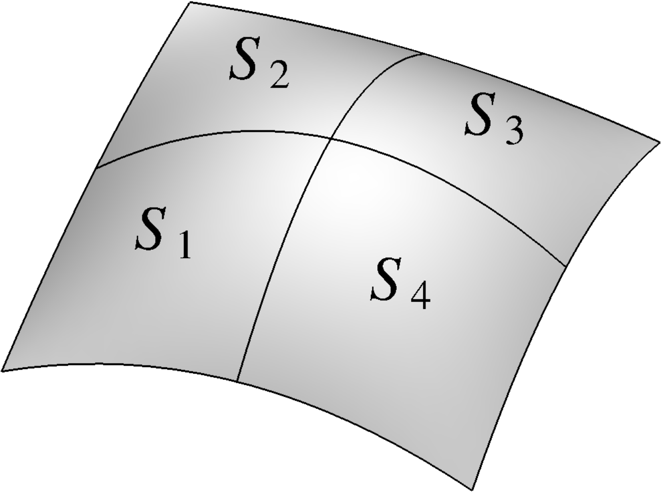 (3.40) For example, in the above figure, the total area of the
overall patch is given by
(3.40) For example, in the above figure, the total area of the
overall patch is given by
(3.40) However, the additive property by
itself is not sufficient for the concept of area. After all, if a surface is curved, then so are
all of its parts. Thus, subdivision of a surface does not eliminate the effects of curvature which
make the concept of area challenging in the first place.
The breakthrough comes from the infinitesimal approach, already known to the ancients, which lies
at the very heart of Calculus. The idea is to increase the number of the constituent pieces to
"infinity" where each piece can be thought of as effectively flat. 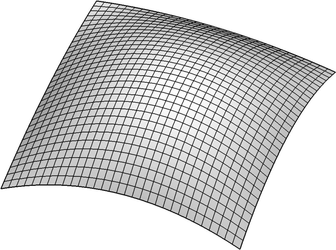 (3.42) What makes the infinitesimal approach work is the fact that,
as the pieces grow in number and their size diminishes, the effects of curvature diminish at a
faster rate. Consequently, when small curved patches are replaced by flat polygons (we omit
the precise details of how to accomplish that), the combined area of the polygons approaches what
we intuitively understand to be the area of the curved surface. This way of reasoning leads to the
following attempt at the definition of area: the area of a curved surface is the limit of the areas
of piecewise flat approximations to the surface as the number of flat pieces increases to infinity
and the size of each piece goes to zero.
(3.42) What makes the infinitesimal approach work is the fact that,
as the pieces grow in number and their size diminishes, the effects of curvature diminish at a
faster rate. Consequently, when small curved patches are replaced by flat polygons (we omit
the precise details of how to accomplish that), the combined area of the polygons approaches what
we intuitively understand to be the area of the curved surface. This way of reasoning leads to the
following attempt at the definition of area: the area of a curved surface is the limit of the areas
of piecewise flat approximations to the surface as the number of flat pieces increases to infinity
and the size of each piece goes to zero.
(3.42)This definition has been known to be deeply problematic ever since the paper by Hermann Schwarz titled On an erroneous
definition of area of a curved surface surprised the mathematical community by showing that the
surface of a cylinder can be approximated by increasingly small triangles whose combined area grows
without bound instead of converging to the area of the cylinder. Thus, at the very least,
additional stipulations are needed on the precise manner in which the piecewise flat "mesh"
approaches the curved surface in order for the area of the former to converge to the area of the
latter. However, these important technical details are beyond our scope. Nevertheless, this and
many other difficulties notwithstanding, the idea of infinite subdivision has more than earned its
place in the mathematical toolbox. While it is important to be aware of the serious difficulties
with which some mathematical concepts present us, it is even more important to develop a habit of
moving forward, all the while contemplating the uncertainties inevitably left behind.
The infinitesimal approach is particularly fitting in the context of our narrative since it is
entirely geometric. It offers an effective way of defining the concepts of length, area, and volume
by a geometric approach that does not require the introduction of coordinates.
3.7Arc length as parameterization of a curve
Arc length, which is a synonym for the length of a curve, offers a convenient way of
parameterizing the curve. Select an arbitrary point on the curve
to serve as a reference point known as the origin and associate with every point its
signed arc length to the point . To define
signed arc length, arbitrarily choose one of the directions along the curve as
positive and the other as negative. Then, to the points along the positive direction,
assign their actual arc length, while to the points along the negative direction, assign
minus their actual arc length. The choice of the direction in which the parameterization
increases is known as its orientation and is entirely analogous to the concept of
orientation in a one-dimensional Euclidean space.  (3.43)
(3.43)We should note that the use of any parameterization amounts to imposing a coordinate system upon
the curve, with an arc length parameterization being a particularly special coordinate system.
Thus, relying on this parameterization is somewhat controversial in the context of Tensor Calculus
which is built on the idea of avoiding special coordinate systems. On the other hand, arc length is
a very natural coordinate system because of its perfect regularity along the curve, and in Chapter
5, it will demonstrate its unique value for some
theoretical investigations. However, it is not well suited for other theoretical investigations as
well as virtually all practical calculations. We will therefore have to later revisit the analysis
of curves with the help of a fully developed tensor framework.
3.8Integration
The idea of infinite subdivision can also be used as the foundation of the theory of integration.
(In fact, the integral sign was
introduced by Gottfried Leibniz as a stylized letter S for sum.) For example, for a
scalar defined on a
domain , the volume integral
newline can be defined as the limit
of the familiar Riemann sum as the
subdivision of the domain increases. The exact same limiting process can be applied to a surface
integral
over a surface patch , as well as a
line integral
over a curve segment . In the above expressions the traditional
symbols , , and represent the
proverbial infinitesimal amounts of length, area, and volume.
Thus, the idea of integration is no more conceptually challenging than that of length, area, or
volume, and we will similarly accept it without a formal definition. Note, furthermore, that
integration works just as effectively for vector fields as it does for scalar fields.
Indeed, for a vector field , the
vector-valued integral
makes sense since geometric vectors
are subject to addition and multiplication by numbers and therefore the Riemann sum is perfectly meaningful.
The interpretation of the integral of a quantity defined on
some domain -- be it a curve, a surface, or a solid -- is straightforward and simple: it is the
total amount of over the
domain. For instance, if is the density distribution of a body occupying a domain
, then the integral
represents the total mass.
Similarly, if is the
electric charge distribution over a surface , then the
integral
represents the total charge. For a
vector-valued example, if is the (variable) acceleration of
gravity distribution with density distribution , then the integral
represents the total force of
gravity. If the integrand is chosen to be , then the curve, surface, and volume integrals yield the
length of the curve, the area of the
surface, and the volume of the solid, i.e.
These nearly tautological formulas will be used with surprising frequency in our future analyses.
In the context of our approach, integrals can be described as invariant since they are
defined strictly in terms of geometric quantities and without the use of coordinate systems. In
fact, a surprising amount of theoretical analysis with integrals can be performed without the use
of specific coordinate systems. Nevertheless, most practical problems do require specific
coordinates and thus, one of the tasks that Tensor Calculus takes upon itself is to provide a
recipe for converting an invariant integral into an coordinate space arithmetic integral that can
be evaluated by the techniques of ordinary Calculus or with the help of computational techniques.
3.9Exercises
Exercise 3.1In both two and three dimensions, show that switching the order of any two vectors in a basis changes its orientation.
Exercise 3.2In a three-dimensional space, show that the sets of vectors , , and have the same orientation, opposite of that shared by the sets , , and .
Exercise 3.3In a three-dimensional space, show that the orientation of the set of vectors is opposite that of .
Exercise 3.4In a three-dimensional space, show that reflecting a basis with respect to a plane changes its orientation. Similarly, in a two-dimensional space, show that reflecting the basis with respect to a straight line changes its orientation.
Exercise 3.5Confirm that the linear independence of the vectors , , and is maintained at each step of the evolution described in Section 3.2.
Exercise 3.6Use an argument analogous to that of Section 3.2 to demonstrate the determinant criterion for matching orientations in the two-dimensional case.
Exercise 3.7Use the determinant criterion to show that adding a multiple of one vector to another does not change the orientation of a basis, while switching the order of two vectors does change the orientation, as does multiplying one of the vectors by a negative number.
Exercise 3.8Demonstrate the associative property
of the cross product by a geometric argument.
Exercise 3.9Suppose that is the cross product of and :
If , , and represent the mirror images of , , and , is the cross product of and ? A mirror image is the result of reflecting a vector with respect to a plane. It is implied that all three vectors , , and are reflected with respect to the same plane.
Exercise 3.11Show by a geometric argument that the combination
equals the signed volume of the parallelepiped formed by the vectors , , and .
Exercise 3.12Alternatively, show that the combination
equals the signed volume of the parallelepiped formed by the vectors , , and by demonstrating that the above product satisfies the three governing properties of signed volume discussed in Section 3.3.
Exercise 3.13From the two preceding exercises, conclude that
Exercise 3.14Use the above identity to prove the distributive property
of the cross product. Hint: Dot the presumed identity with an arbitrary vector .