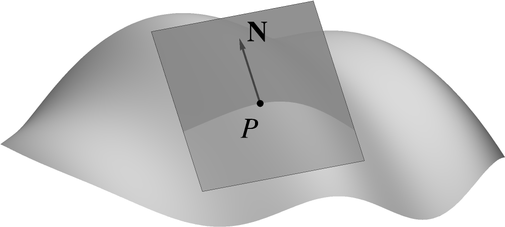
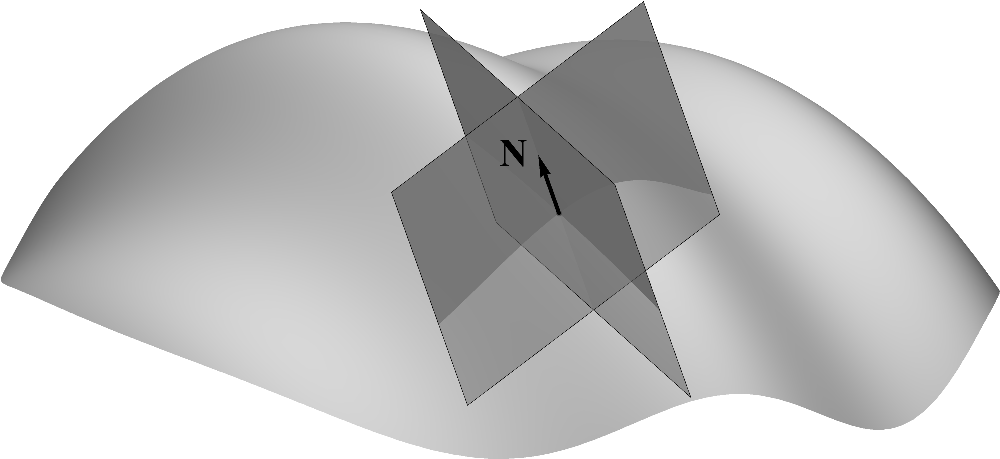
This entire Chapter is devoted to the exploration of the curvature tensor \(B_{\alpha\beta}\). We
will begin by recalling the key relationships involving the curvature tensor \(B_{\alpha\beta}\)
that we have established in the earlier Chapters.
6.1Elementary identities and definitions
Our analytical exploration of curvature started with the realization that the spatial variability
of the surface covariant basis \(\mathbf{S}_{\alpha}\) comes from two sources: the potential
non-uniformity of the surface coordinates \(S^{\alpha}\) and the non-flatness -- in other words,
curvature -- of the surface. While the non-uniformity of the surface coordinates can be
effectively managed by switching from partial to covariant differentiation, the curvature of the
surface is a matter of actual geometry. We therefore embrace it rather than seek to eliminate it
from consideration by some analytical device.
The opportunity to quantify curvature presented itself when we discovered that each of the vectors
in the tensor \(\nabla_{\alpha}\mathbf{S}_{\beta}\) is orthogonal to the surface and therefore
collinear with the unit normal \(\mathbf{N}\). We then assembled corresponding coefficients of
proportionality into a second-order system called the curvature tensor \(B_{\alpha \beta}\),
i.e.
\[
\nabla_{\alpha}\mathbf{S}_{\beta}=\mathbf{N}B_{\alpha\beta}. \tag{2.79}
\]
Dotting both sides of the above equation with \(\mathbf{N}\) yields an explicit expression
for \(B_{\alpha\beta}\) captured by the equation
\[
B_{\alpha\beta}=\mathbf{N}\cdot\nabla_{\alpha}\mathbf{S}_{\beta}. \tag{2.80}
\]
Since the covariant basis \(\mathbf{S}_{\beta}\) is the derivative of the position vector
\(\mathbf{R}\), i.e.
\[
\mathbf{S}_{\beta}=\nabla_{\beta}\mathbf{R,}\tag{6.1}
\]
the above identities may also be written in forms
\[
\nabla_{\alpha}\nabla_{\beta}\mathbf{R}=\mathbf{N}B_{\alpha\beta}.\tag{6.2}
\]
and
\[
B_{\alpha\beta}=\mathbf{N}\cdot\nabla_{\alpha}\nabla_{\beta}\mathbf{R}\tag{6.3}
\]
in terms of the second derivatives of \(\mathbf{R}\). Note that while, in general, the
covariant derivatives \(\nabla_{\alpha}\) and \(\nabla_{\beta}\) do not commute, they do
commute when applied to a variant of order zero. Indeed, for a zeroth-order variant \(U\), we have
\[
\nabla_{\alpha}\nabla_{\beta}U=\frac{\partial^{2}U}{\partial S^{\alpha }\partial
S^{\beta}}-\Gamma_{\alpha\beta}^{\omega}\frac{\partial U}{\partial S^{\omega}}.\tag{6.4}
\]
Since the Christoffel symbol is symmetric in its subscripts, i.e.
\[
\Gamma_{\alpha\beta}^{\gamma}=\Gamma_{\beta\alpha}^{\gamma},\tag{6.5}
\]
both of the terms in the expression for \(\nabla_{\alpha}\nabla_{\beta}U\) are symmetric in
\(\alpha\) and \(\beta\) and therefore
\[
\nabla_{\alpha}\nabla_{\beta}U=\nabla_{\beta}\nabla_{\alpha}U.\tag{6.6}
\]
Therefore \(\nabla_{\alpha}\nabla_{\beta}\mathbf{R}\) is symmetric, i.e.
\[
\nabla_{\alpha}\nabla_{\beta}\mathbf{R}=\nabla_{\beta}\nabla_{\alpha }\mathbf{R.}\tag{6.7}
\]
In other words,
\[
\nabla_{\alpha}\mathbf{S}_{\beta}=\nabla_{\beta}\mathbf{S}_{\alpha}, \tag{2.78}
\]
from which it follows that the curvature tensor \(B_{\alpha\beta}\) is symmetric, i.e.
\[
B_{\alpha\beta}=B_{\beta\alpha} \tag{2.81}
\]
or, equivalently,
\[
B_{\cdot\beta}^{\alpha}=B_{\beta}^{\cdot\alpha}. \tag{2.82}
\]
Because of the symmetry of the curvature tensor, its mixed form
\[
B_{\beta}^{\alpha}\tag{6.8}
\]
can be written in this simplified form without the use of the dot placeholder. This subtle
point was discussed in Chapter TBD of Introduction to Tensor Calculus. Finally, recall that,
as we discussed in Chapter 2, the covariant
derivative in the identity
\[
B_{\alpha\beta}=\mathbf{N}\cdot\nabla_{\alpha}\mathbf{S}_{\beta} \tag{2.80}
\]
may be replaced with the partial derivative, i.e.
\[
B_{\alpha\beta}=\mathbf{N}\cdot\frac{\partial\mathbf{S}_{\beta}}{\partial S^{\alpha}}. \tag{2.83}
\]
In Chapter 5, we observed that \(B_{\alpha\beta}\)
can be computed in the component space by the equation
\[
B_{\alpha\beta}=N_{i}\nabla_{\alpha}Z_{\beta}^{i} \tag{5.54}
\]
and the Weingarten equation
\[
B_{\alpha\beta}=-Z_{\beta}^{i}\nabla_{\alpha}N_{i}, \tag{5.55}
\]
where \(Z_{\beta}^{i}\) is the shift tensor obtained by differentiating the equations of the
surface \(Z^{i}\left( S\right) \), i.e.
\[
Z_{\alpha}^{i}=\frac{\partial Z^{i}\left( S\right) }{\partial S^{\alpha}}. \tag{3.68}
\]
Importantly, the "sign" of the curvature tensor depends on the choice of normal. Recall that there
are two unit normals pointing in opposite directions and, as we agreed in Chapter 2, the symbol \(\mathbf{N}\) represents either one of
them. Thus, depending on the choice of normal, the resulting elements in the tensor
\(B_{\alpha\beta}\) may summarily change sign. As a result, the curvature tensor inherits the same
sign ambiguity of the unit normal. By extension, the same is true of the mean curvature \(B_{\alpha
}^{\alpha}\). The Gaussian curvature \(K\), on the other hand, being the determinant of the
\(2\times2\) matrix corresponding to \(B_{\beta}^{\alpha}\), is unchanged when the sign of the
matrix is flipped and is therefore independent of the choice of normal. The product
\(\mathbf{N}B_{\alpha\beta}\), known as the vector curvature tensor, is also independent of
the choice of normal since both elements in the product change sign when the normal is reversed.
6.2The invariants of the curvature tensor
This Section calls for a brief Linear Algebra preamble. As we described in Chapter TBD of
Introduction to Tensor Calculus, a matrix \(A\) representing a linear transformation
corresponds to a mixed second-order tensor \(A_{\cdot\beta}^{\alpha}\). Such a matrix \(A\) is
characterized by \(n\) fundamental invariants -- its eigenvalues \(\lambda_{1}\), \(\lambda_{2}\),
\(\cdots\), \(\lambda_{n}\). From these invariants, numerous others can be constructed. Two of the
most noteworthy such invariants are the sum of the eigenvalues, which equals the trace of
\(A\), i.e.
\[
\operatorname{trace}\left( A\right) =\lambda_{1}+\lambda_{2}+\cdots +\lambda_{n},\tag{6.9}
\]
and their product, which equals the determinant, i.e.
\[
\det\left( A\right) =\lambda_{1}\lambda_{2}\cdots\lambda_{n}.\tag{6.10}
\]
While the eigenvalues of a general \(n\times n\) matrix may be difficult to calculate (in
fact, no finite algorithm for calculating eigenvalues is possible for a matrix of dimension greater
than \(4\)), the trace and the determinant are readily available.
For a self-adjoint transformation characterized by a symmetric tensor \(A_{\cdot\beta}^{\alpha}\),
i.e.
\[
A_{\cdot\beta}^{\alpha}=A_{\beta}^{\cdot\alpha},\tag{6.11}
\]
all eigenvalues are real and the corresponding eigenvectors are orthogonal -- or, in the
case of repeated eigenvalues, can be chosen to be orthogonal. The eigenvectors represent the
critical points of the quadratic form
\[
F\left( U\right) =A_{\alpha\beta}U^{\alpha}U^{\beta},\tag{6.12}
\]
subject to the unit-length constraint
\[
S_{\alpha\beta}U^{\alpha}U^{\beta}=1.\tag{6.13}
\]
When we transfer these facts onto the curvature tensor \(B_{\beta}^{\alpha}\), we find that each of
the objects mentioned above are of great geometric importance. The eigenvalues \(\kappa_{1}\) and
\(\kappa_{2}\) are known as the principal curvatures while the corresponding eigenvectors
are known as the principal directions. The sum \(\kappa_{1}+\kappa_{2}\) is, of course, the
mean curvature \(B_{\alpha}^{\alpha}\) while their product \(\kappa_{1}\kappa_{2}\) is, of
course, the Gaussian curvature. We will now take a detailed look into each of these
elements, starting with mean curvature.
6.2.1The mean curvature
The invariant
\[
B_{\alpha}^{\alpha}\tag{6.14}
\]
is known as the mean curvature of the surface. The mean curvature is often denoted by
the letter \(\kappa\) but we will almost always prefer the symbol \(B_{\alpha}^{\alpha}\).
The mean curvature is a particularly important invariant that appears in many fundamental
identities. It is, by virtue of its ubiquity, the star of our entire narrative. Many physical
phenomena associated with capillary pressure (i.e. the pressure differential across an interface
between two fluids) are described by equations that invariably feature the mean curvature. Thus,
not surprisingly, it plays an important role in the dynamics of fluid films. Furthermore, mean
curvature plays an important role in the study of minimal surfaces, i.e. surfaces with a
given boundary that have the least possible area. As we will demonstrate in a future book on the
Calculus of Moving Surfaces, minimal surfaces are characterized by zero mean curvature.
The vector \(\mathbf{N}B_{\alpha}^{\alpha}\) can be referred to as the vector mean curvature
or, by analogy with curves that we will discover in Chapter 8, as the curvature normal. As we learned in Chapter 2, it equals the surface divergence of the covariant
basis \(\mathbf{S}^{\alpha}\) or the surface Laplacian of the position vector \(\mathbf{R}\), i.e.
\[
\mathbf{N}B_{\alpha}^{\alpha}=\nabla_{\alpha}\mathbf{S}^{\alpha}
=\nabla_{\alpha}\nabla^{\alpha}\mathbf{R.}\tag{6.15}
\]
Thus, an alternative expression for the mean curvature is
\[
B_{\alpha}^{\alpha}=\mathbf{N}\cdot\nabla_{\alpha}\nabla^{\alpha}\mathbf{R.}\tag{6.16}
\]
The advantage of these identities is, of course, their pure geometric nature. For example,
the first of the two equations will readily explain why the integral of the curvature normal over a
closed surface is zero.
6.2.2The Gaussian curvature
The determinant \(B\) of the mixed curvature tensor \(B_{\beta}^{\alpha}\) of a two-dimensional
surface is the Gaussian curvature \(K\). However, this is not the definition of
Gaussian curvature but rather a consequence of the Gauss equations which we mentioned in
Chapter 2 and will describe in detail in Chapter 7. As we stated in Chapter 2, by definition, the Gaussian curvature is the invariant \(K\) in
the two-dimensional identity
\[
R_{\alpha\beta\gamma\delta}=K\varepsilon_{\alpha\beta}\varepsilon _{\gamma\delta}. \tag{7.51}
\]
where \(R_{\alpha\beta\gamma\delta}\) is the Riemann-Christoffel tensor. Meanwhile, as we
showed in Chapter TBD of Introduction to Tensor Calculus, any second-order system
\(B_{\beta}^{\alpha}\) in a two-dimensional space satisfies the equation
\[
B_{\alpha\gamma}B_{\beta\delta}-B_{\alpha\delta}B_{\beta\gamma}=B\varepsilon
_{\alpha\beta}\varepsilon_{\gamma\delta}.\tag{6.17}
\]
Now, this is where the Gauss equations enter. From the Gauss equations
\[
B_{\alpha\gamma}B_{\beta\delta}-B_{\alpha\delta}B_{\beta\gamma}=R_{\alpha \beta\gamma\delta}
\tag{7.38}
\]
we conclude that
\[
B\varepsilon_{\alpha\beta}\varepsilon_{\gamma\delta}=K\varepsilon_{\alpha
\beta}\varepsilon_{\gamma\delta}\tag{6.18}
\]
and therefore
\[
K=B. \tag{7.60}
\]
We will save the rest of our discussion of Gaussian curvature for Chapter 7.
6.2.3The principal curvatures
The eigenvalues of \(B_{\beta}^{\alpha}\) are known as the principal curvatures. Thus,
two-dimensional surfaces are characterized by two eigenvalues, \(\kappa_{1}\) and \(\kappa_{2}\).
As mentioned earlier, the principal curvatures \(\kappa_{1}\) and \(\kappa_{2}\) correspond to the
minimum and the maximum values of the quadratic form
\[
B_{\alpha\beta}X^{\alpha}X^{\beta}\tag{6.19}
\]
subject to the unit normalization condition
\[
S_{\alpha\beta}X^{\alpha}X^{\beta}=1.\tag{6.20}
\]
Furthermore their sum is the mean curvature, i.e.
\[
B_{\alpha}^{\alpha}=\kappa_{1}+\kappa_{2}.\tag{6.21}
\]
and their product is the determinant \(B\) of \(B_{\beta}^{\alpha}\) which, by the Gauss
equations, equals the Gaussian curvature \(K\), i.e.
\[
K=B=\kappa_{1}\kappa_{2}. \tag{7.61}
\]
The geometric interpretation of the principal curvatures \(\kappa_{1}\) and \(\kappa_{2}\)
and the corresponding eigenvectors will be described below in a Section devoted entirely to that
topic.
Note that some texts define the mean curvature as the average of the principal curvatures,
i.e.
\[
\frac{\kappa_{1}+\kappa_{2}}{2},\tag{6.22}
\]
which explains the use of the word mean in mean curvature. Such a definition
has some advantages over our definition. For example, as we demonstrate below, the mean curvature
\(B_{\alpha}^{\alpha}\) of a sphere of radius \(R\) is \(-2/R\) which, in \(n\) dimensions,
generalizes to \(-n/R\). The definition based on the average, on the other hand, yields the value
of \(-1/R\) in all dimensions. Nevertheless, we will stick with our definition since, in numerous
applications, including the Calculus of Moving Surfaces, it is \(B_{\alpha}^{\alpha}\), rather than
\(B_{\alpha}^{\alpha}/2\), that is most frequently encountered.
6.2.4The third fundamental tensor of a surface
The metric tensor \(S_{\alpha\beta}\) is sometimes referred to as the first fundamental
tensor of the surface while the curvature tensor \(B_{\alpha\beta}\) is referred to as the
second fundamental tensor. The third fundamental tensor \(C_{\beta}^{\alpha}\), which
arises frequently in applications, is the tensor \(C_{\beta}^{\alpha}\) defined by the equation
\[
C_{\beta}^{\alpha}=B_{\gamma}^{\alpha}B_{\beta}^{\gamma}.\tag{6.23}
\]
In other words, \(C_{\beta}^{\alpha}\) corresponds to the matrix square of the curvature
tensor. Note that the fundamental tensors often figure as binlinear forms, such as
\(S_{\alpha\beta}U^{\alpha}V^{\beta}\). For this reason, they can also be referred to as
fundamental forms or groundforms.
It is left as an exercise to show that
\[
\nabla_{\alpha}\mathbf{N}\cdot\nabla_{\beta}\mathbf{N}=C_{\alpha\beta}\tag{6.24}
\]
Note the similarity among the equations that can act as definitions of the first groundform
\(S_{\alpha\beta}\), the second groundform \(B_{\alpha\beta}\), and the third groundform
\(C_{\alpha\beta}\), especially if we denote \(\mathbf{S}_{\alpha}=\nabla_{\alpha}\mathbf{R}\) by
\(\mathbf{R}_{\alpha}\) and \(\nabla_{\alpha}\mathbf{N}\) by \(\mathbf{N}_{\alpha}\). Then we have
\[
\begin{aligned}
S_{\alpha\beta} & =\mathbf{R}_{\alpha}\cdot\mathbf{R}_{\beta}\ \ \ \ \ \ \ \ \ \
\left(6.25\right)\\
-B_{\alpha\beta} & =\mathbf{N}_{\alpha}\cdot\mathbf{R}_{\beta}\ \ \ \ \ \ \ \ \ \
\left(6.26\right)\\
C_{\alpha\beta} & =\mathbf{N}_{\alpha}\cdot\mathbf{N}_{\beta}.\ \ \ \ \ \ \ \ \ \
\left(6.27\right)
\end{aligned}
\]
As we know from Linear Algebra, the eigenvalues of \(C_{\beta}^{\alpha}\) are
\(\kappa_{1}^{2},\kappa_{2}^{2},\cdots,\kappa_{n}^{2}\). Therefore, the invariant
\(C_{\alpha}^{\alpha}\) is given by
\[
C_{\alpha}^{\alpha}=\kappa_{1}^{2}+\kappa_{2}^{2}+\cdots+\kappa_{n}^{2},\tag{6.28}
\]
while the determinant \(C\) of \(C_{\beta}^{\alpha}\) is given by
\[
C=\kappa_{1}^{2}\kappa_{2}^{2}\cdots\kappa_{n}^{2}.\tag{6.29}
\]
6.2.5The special case of planar curves
We have already studied planar curves in Chapter TBD of Introduction to Tensor Caclulus,
where our analysis was based on parameterizing the curve by the arc length \(s\). We will now
approach curves from a different angle -- that is, as a special one-dimensional case of an embedded
surface. In other words, we will, to the extent possible, ignore their one-dimensional nature and
focus on what the general theory of surfaces can tell us about them.
A planar curve is a curve embedded in a Euclidean space. Therefore, the dimension of a planar curve
trails that of its ambient space by \(1\), which makes it a hypersurface. As a hypersurface, it is
characterized by a unique (within sign) unit normal \(\mathbf{N}\). Thus, the concept of the
curvature tensor applies in full force, as is the concept of mean curvature. The curvature tensor
\(B_{\alpha\beta}\) is still defined by the equation
\[
\nabla_{\alpha}\mathbf{S}_{\beta}=\mathbf{N}B_{\alpha\beta} \tag{2.79}
\]
or, equivalently,
\[
B_{\alpha\beta}=\mathbf{N}\cdot\nabla_{\alpha}\mathbf{S}_{\beta}, \tag{2.80}
\]
while the mean curvature \(B_{\alpha}^{\alpha}\) is given by
\[
\nabla_{\alpha}\mathbf{S}^{\alpha}=\mathbf{N}B_{\alpha}^{\alpha}\tag{6.30}
\]
or, equivalently,
\[
B_{\alpha}^{\alpha}=\mathbf{N}\cdot\nabla_{\alpha}\mathbf{S}^{\alpha}. \tag{2.80}
\]
Compare this equation to the identity
\[
\kappa=\mathbf{N}\cdot\mathbf{T}^{\prime}\left( s\right)\tag{6.31}
\]
from Chapter TBD of Introduction to Tensor Caclulus, where \(\kappa\) is signed
curvature and \(\mathbf{T}\left( s\right) \) is the unit tangent as a function of the arc
length \(s\). Since, as it is left as an exercise to show, \(\nabla_{\alpha}\mathbf{S}^{\alpha}\)
is equivalent to \(\mathbf{T}^{\prime}\left( s\right) \), we observe that for planar curves, the
concept of mean curvature is equivalent to that of signed curvature.
Below, we will calculate the curvature tensor as well as the mean curvature for general planar
curves represented in Cartesian and polar coordinates.
6.3The geometric interpretation of the principal curvatures
The geometric interpretation of principal curvatures involves curves embedded in two-dimensional
surfaces. This configuration creates a fascinating interplay among three spaces: the
one-dimensional curve, the two-dimensional surface, and the three-dimensional ambient Euclidean
space. This intricate arrangement will yield a great number of intriguing relationships and
insights. Some of these will appear in this book, but a great many more are beyond our scope -- and
many more still are yet to be discovered.
Note that we have not yet developed a theory of surfaces embedded in non-Euclidean spaces, which is
what a curve embedded in a general two-dimensional surface represents. Such a theory will be
developed in Chapter 9. Fortunately, in order to
understand the geometric interpretation of principal curvatures, we will only need to consider
planar curves which, as we saw in the previous Section, we already have under our belt.
A planar curve arises when a surface is cut by a plane, as illustrated in the following figure.
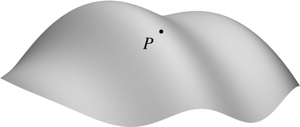
(6.32)
Our analysis will focus on a single point \(P\) which lies on
the curve at the intersection of the surface and the cutting plane. Furthermore, we will assume
that the cutting plane is orthogonal to the surface at the point \(P\). In other words, the
cutting plane contains within in it the surface normal \(\mathbf{N}\) at \(P\). (6.33)
This condition does not specify the plane uniquely as there is
an entire family of such planes obtained by rotation about the straight line containing
\(\mathbf{N}\).
The curve at the intersection of the surface and the plane can be analyzed from three distinct
points of view. First, it can be viewed as a curve embedded in the two-dimensional surface. In this
context, the surface can be described as the ambient space with respect to the curve.
Second, it can be viewed as a curve embedded in the overall three-dimensional Euclidean space. And
finally, it can be viewed as a curve embedded in the two-dimensional Euclidean cutting plane.
Naturally, it is the last embedding with which we will concern ourselves here.
The curve represents a hypersurface with the respect to the plane. It is therefore characterized by
its signed curvature \(\kappa\) which, as we observed in the previous section, is equivalent
to its mean curvature in the context of its embedding in the plane. Naturally, \(\kappa\) depends
on two characteristics: the curvature characteristics of the ambient surface and the orientation of
the cutting plane. In this Section, we will succeed in capturing these dependencies by the elegant
equation
\[
\kappa=B_{\alpha\beta}T^{\alpha}T^{\beta},\tag{6.34}
\]
where \(T^{\alpha}\) are the surface components of the unit tangent \(\mathbf{T}\) to the
curve. Clearly, the curvature tensor \(B_{\alpha\beta}\) captures the curvature characteristics of
the surface while the tangent \(\mathbf{T}\) captures the orientation of the surface. The reader is
invited to attempt deriving this identity on their own before we lay out the details below, as it
relies on the techniques that we have developed earlier.
Before we turn to the derivation of the above identity, let us make one important geometric
observation that will prove relevant later. Consider the unit normal \(\mathbf{\tilde{N}}\) to the
curve when viewed as a hypersurface within the cutting plane. At the point \(P\), and likely
only at the point \(P\), it is colinear with the surface normal \(\mathbf{N}\). This is by
construction: the surface normal \(\mathbf{N}\) at the point \(P\) is orthogonal to all
curves in the surface that pass through \(P\), including the one formed by the intersection of the
surface and the plane. The same cannot be said for any other point on the curve since there is no
guarantee that the surface normal is contained within the cutting plane.
Despite our present affinity for treating curves as a special case of surfaces, we will, for the
remainder of this Section, return to the style of analysis based on parameterizing the curve by its
arc length \(s\), which we employed in Chapter TBD of Introduction to Tensor Calculus. As
before, denote the function representing the position vector \(\mathbf{R}\) at the points on the
curve by \(\mathbf{R}\left( s\right) \), i.e.
\[
\mathbf{R}=\mathbf{R}\left( s\right) .\tag{6.35}
\]
Recall that the first derivative of \(\mathbf{R}\left( s\right) \) is the unit tangent
\(\mathbf{T}\), i.e.
\[
\mathbf{T}=\mathbf{R}^{\prime}\left( s\right) ,\tag{6.36}
\]
while the second derivative is the curvature normal \(\mathbf{B}\), i.e.
\[
\mathbf{B}=\mathbf{R}^{\prime\prime}\left( s\right) .\tag{6.37}
\]
(Note that the determinant \(B\) of the surface curvature tensor \(B_{\beta }^{\alpha}\) is
unrelated to the magnitude of the vector \(\mathbf{B}\).) Importantly, for all \(s\), the vectors
\(\mathbf{T}\left( s\right) \) and \(\mathbf{B}\left( s\right) \) both lie within the cutting
plane. Meanwhile, the curvature normal \(\mathbf{B}\) is collinear with the in-plane normal
\(\mathbf{\tilde{N}}\) to the curve which coincides with the surface normal \(\mathbf{N}\) at the
point \(P\). Thus, at the point \(P\), the signed curvature \(\kappa\), given by the identity
\[
\mathbf{B}=\kappa\mathbf{\tilde{N},}\tag{6.38}
\]
is also given by the identity
\[
\mathbf{B}=\kappa\mathbf{N.}\tag{6.39}
\]
All but the last equation in the previous paragraph are characteristic of the curve with respect to
its embedding in the cutting plane. Thus, in order to derive the equation
\[
\kappa=B_{\alpha\beta}T^{\alpha}T^{\beta}, \tag{6.34}
\]
we must find a meaningful way to engage the differential characteristic of the surface.
Suppose that the curve within the surface is given by the equations
\[
S^{\alpha}=S^{\alpha}\left( s\right) .\tag{6.40}
\]
Then the function \(\mathbf{R}\left( s\right) \) can be constructed by composing the
function \(\mathbf{R}\left( S\right) \), i.e. \(\mathbf{R}\) as a function of the surface
coordinates \(S^{\alpha}\), with the equations of the curve \(S^{\alpha}\left( s\right) \), i.e.
\[
\mathbf{R}\left( s\right) =\mathbf{R}\left( S\left( s\right) \right) .\tag{6.41}
\]
As we always do after establishing a relationship such as above, we will differentiate both
sides with respect to the independent variable, i.e. the arc length \(s\). By the chain rule, we
have
\[
\mathbf{R}^{\prime}\left( s\right) =\frac{\partial\mathbf{R}\left( S\right) }{\partial
S^{\alpha}}\frac{dS^{\alpha}\left( s\right) }{ds}.\tag{6.42}
\]
On the left, we recognize \(\mathbf{R}^{\prime}\left( s\right) \) as the unit tangent
\(\mathbf{T}\). On the right, the partial derivative \(\partial \mathbf{R}\left( S\right)
/\partial S^{\alpha}\) is, of course, the surface covariant basis \(\mathbf{S}_{\alpha}\). In other
words, we have obtained the identity
\[
\mathbf{T}=\frac{dS^{\alpha}\left( s\right) }{ds}\mathbf{S}_{\alpha}\tag{6.43}
\]
which tells us that the derivatives
\[
\frac{dS^{\alpha}\left( s\right) }{ds}\tag{6.44}
\]
of the equations of the curve \(S^{\alpha}\left( s\right) \) can be interpreted as the
surface coordinates \(T^{\alpha}\) of \(\mathbf{T}\). In this respect, the equation
\[
\mathbf{T}=\frac{dS^{\alpha}\left( s\right) }{ds}\mathbf{S}_{\alpha} \tag{6.43}
\]
is similar to a number of identities we have derived in the past, such as
\[
\mathbf{V}=\frac{dZ^{i}\left( t\right) }{dt}\mathbf{Z}_{i}\tag{6.45}
\]
in Chapter TBD of Introduction to Tensor Calculus.
In order to get to curvature, we must differentiate the identity
\[
\mathbf{T}\left( s\right) =\frac{dS^{\alpha}\left( s\right) } {ds}\mathbf{S}_{\alpha}\left(
s\right) \tag{6.43}
\]
a second time. By the product rule,
\[
\mathbf{T}^{\prime}\left( s\right) =\frac{d^{2}S^{\alpha}\left( s\right)
}{ds^{2}}\mathbf{S}_{\alpha}+\frac{dS^{\alpha}\left( s\right) }{ds}
\frac{d\mathbf{S}_{\alpha}\left( s\right) }{ds}.\tag{6.46}
\]
As we recalled above, the derivative \(\mathbf{T}^{\prime}\left( s\right) \) is the
curvature normal \(\mathbf{B}\). Meanwhile, on the right, the object of utmost interest is the
derivative
\[
\frac{d\mathbf{S}_{\alpha}\left( s\right) }{ds}\tag{6.47}
\]
which captures the rate of change of the covariant surface basis \(\mathbf{S}_{\alpha}\)
along the curve. Similarly to \(\mathbf{R}\left( s\right) \), the function
\(\mathbf{S}_{\alpha}\left( s\right) \) can be constructed by substituting the equations of the
curve \(S^{\alpha}=S^{\alpha }\left( s\right) \) into \(\mathbf{S}_{\alpha}\left( S\right) \),
i.e.
\[
\mathbf{S}_{\alpha}\left( s\right) =\mathbf{S}_{\alpha}\left( S\left( s\right) \right)
.\tag{6.48}
\]
Then, by the chain rule, we have
\[
\frac{d\mathbf{S}_{\alpha}\left( s\right) }{ds}=\frac{\partial \mathbf{S}_{\alpha}\left(
S\right) }{\partial S^{\beta}}\frac{dS^{\beta }\left( s\right) }{ds}.\tag{6.49}
\]
The derivative \(\partial\mathbf{S}_{\alpha}\left( S\right) /dS^{\beta}\) is where the
curvature tensor makes its appearance. Since
\[
\nabla_{\beta}\mathbf{S}_{\alpha}=\mathbf{N}B_{\alpha\beta}, \tag{2.79}
\]
and by definition of the covariant derivative
\[
\nabla_{\beta}\mathbf{S}_{\alpha}=\frac{\partial\mathbf{S}_{\alpha}\left( S\right) }{\partial
S_{\beta}}-\Gamma_{\alpha\beta}^{\omega}\mathbf{S} _{\omega},\tag{6.50}
\]
we find
\[
\frac{\partial\mathbf{S}_{\alpha}\left( S\right) }{\partial S^{\beta}
}=\mathbf{N}B_{\alpha\beta}+\Gamma_{\alpha\beta}^{\omega}\mathbf{S}_{\omega}.\tag{6.51}
\]
Thus,
\[
\frac{d\mathbf{S}_{\alpha}\left( s\right) }{ds}=\frac{\partial \mathbf{S}_{\alpha}\left(
S\right) }{\partial S^{\beta}}\frac{dS^{\beta }\left( s\right) }{ds}\tag{6.52}
\]
becomes
\[
\frac{d\mathbf{S}_{\alpha}\left( s\right) }{ds}=\left( \mathbf{N}
B_{\alpha\beta}+\Gamma_{\alpha\beta}^{\omega}\mathbf{S}_{\omega}\right)
\frac{dS^{\beta}}{ds}\tag{6.53}
\]
and therefore
\[
\mathbf{T}^{\prime}\left( s\right) =\frac{d^{2}S^{\alpha}\left( s\right)
}{ds^{2}}\mathbf{S}_{\alpha}+\frac{dS^{\alpha}\left( s\right) }{ds}
\frac{d\mathbf{S}_{\alpha}\left( s\right) }{ds} \tag{6.46}
\]
becomes
\[
\mathbf{B}=\left( \mathbf{N}B_{\alpha\beta}+\Gamma_{\alpha\beta}^{\omega
}\mathbf{S}_{\omega}\right) \frac{dS^{\alpha}}{ds}\frac{dS^{\beta}}
{ds}+\mathbf{S}_{\alpha}\frac{d^{2}S^{\alpha}}{ds^{2}}\tag{6.54}
\]
where we have dropped the arguments of the functions for the sake of conciseness. Combining
normal and tangential terms, we find
\[
\mathbf{B}=\mathbf{N}B_{\alpha\beta}\frac{dS^{\alpha}}{ds}\frac{dS^{\beta} }{ds}+\left(
\frac{d^{2}S^{\alpha}}{ds^{2}}+\Gamma_{\beta\omega}^{\alpha
}\frac{dS^{\beta}}{ds}\frac{dS^{\omega}}{ds}\right) \mathbf{S}_{\alpha}.\tag{6.55}
\]
On the one hand, the combination
\[
\frac{d^{2}S^{\alpha}}{ds^{2}}+\Gamma_{\beta\omega}^{\alpha}\frac{dS^{\beta}
}{ds}\frac{dS^{\omega}}{ds},\tag{6.56}
\]
which represents the tangential component of the curvature normal \(\mathbf{B} \), is quite
intriguing as it reminds us of the \(\delta/\delta t\)-derivative introduced in Section TBD of
Introduction to Tensor Calculus. It will also reemerge in the future as we study the concept
of the geodesic curvature for curves embedded in surfaces. On the other hand, since the curvature
normal \(\mathbf{B}\) is colinear with the surface normal \(\mathbf{N}\) at the point \(P\) as we
established above, we can conclude that the tangential component of \(\mathbf{B}\) vanishes, i.e.
\[
\frac{d^{2}S^{\alpha}}{ds^{2}}+\Gamma_{\beta\omega}^{\alpha}\frac{dS^{\beta}
}{ds}\frac{dS^{\omega}}{ds}=0.\tag{6.57}
\]
Therefore, the curvature normal \(\mathbf{B}\) is given by
\[
\mathbf{B}=\mathbf{N}B_{\alpha\beta}\frac{dS^{\alpha}}{ds}\frac{dS^{\beta} }{ds}.\tag{6.58}
\]
Finally, since
\[
\mathbf{B}=\kappa\mathbf{N,} \tag{6.39}
\]
we arrive at the identity
\[
\kappa=B_{\alpha\beta}\frac{dS^{\alpha}}{ds}\frac{dS^{\beta}}{ds}.\tag{6.59}
\]
In other words,
\[
\kappa=B_{\alpha\beta}T^{\alpha}T^{\beta}, \tag{6.34}
\]
as we set out to show.
The geometric interpretation of the principal curvatures \(\kappa_{1}\) and \(\kappa_{2}\) follows
immediately from the identity
\[
\kappa=B_{\alpha\beta}T^{\alpha}T^{\beta} \tag{6.34}
\]
Recall that the principal curvatures \(\kappa_{1}\) and \(\kappa_{2}\) of a surface are
defined as the eigenvalues of \(B_{\beta}^{\alpha}\). From Linear Algebra, we know that these
values are precisely the least and greatest values of the quadratic form
\[
B_{\alpha\beta}T^{\alpha}T^{\beta}\tag{6.60}
\]
subject to the constraint
\[
S_{\alpha\beta}T^{\alpha}T^{\beta}=1.\tag{6.61}
\]
Therefore, the principal curvatures correspond to the least and the greatest signed
curvatures of curves formed by intersecting the surface with orthogonal planes. Such values always
exist and the corresponding directions, characterized by the unit tangents \(\mathbf{T}_{1}\) and
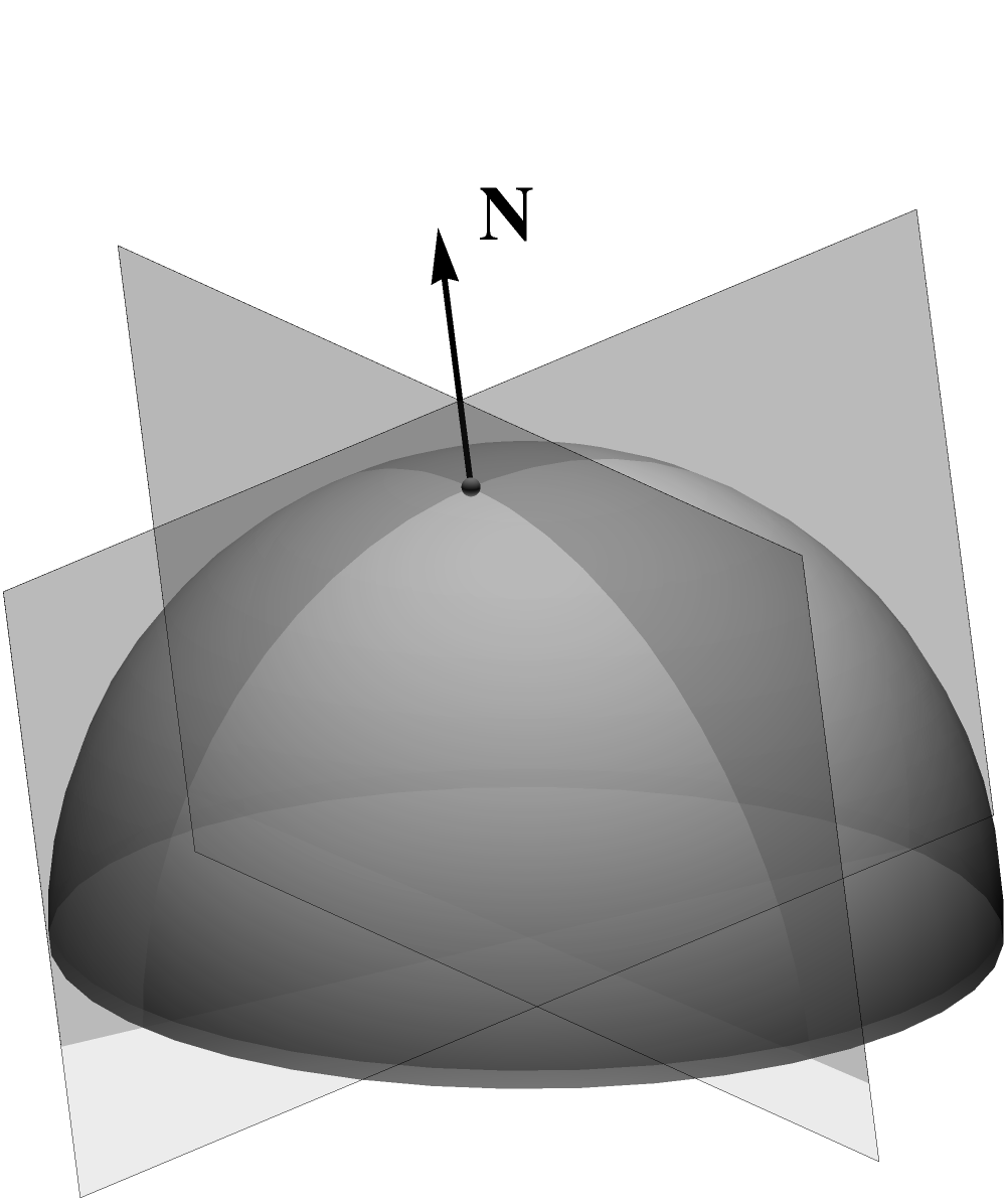
\(\mathbf{T}_{2}\) are orthogonal. The following figure shows the two cutting planes corresponding
to the principal directions. (6.62)
The following figure shows a point where the interplay between
the principal curvatures is more interesting -- one is positive and the other is negative. (6.63)
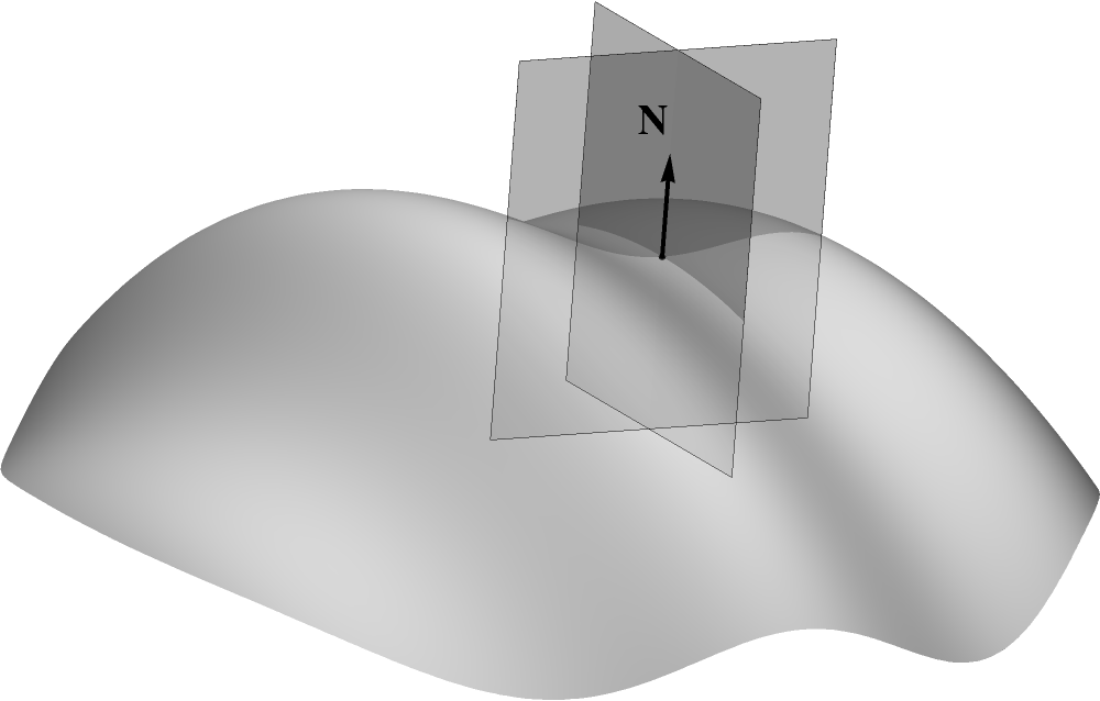
This interpretation of the principal curvatures immediately tells us the curvature invariants on
the sphere of radius \(R\).
(6.64)
A
normal plane cuts the sphere in a great circle of radius \(R\). Thus, with respect to the outward
normal, for both principal curvatures, we have
\[
\kappa_{1}=\kappa_{2}=-\frac{1}{R}.\tag{6.65}
\]
Thus, the mean curvature of the sphere with radius \(R\) with respect to the outward normal
is given by
\[
B_{\alpha}^{\alpha}=\kappa_{1}+\kappa_{2}=-\frac{2}{R}.\tag{6.66}
\]
The Gaussian curvature \(K\), which is independent of the choice of normal, is given by
\[
K=\kappa_{1}\kappa_{2}=\frac{1}{R^{2}}.\tag{6.67}
\]
6.4Calculation of the curvature tensor for several two-dimensional surfaces
In this Section, we will expand the analyses presented in Chapter 4 to include the curvature tensor. One of the more convenient ways to
calculate the curvature tensor by hand is represented by the form
\[
B_{\alpha\beta}=-Z_{\beta}^{i}\nabla_{\alpha}N_{i}, \tag{5.55}
\]
of Weingarten's equation. When the ambient space is referred to Cartesian coordinates,
\(\nabla_{\alpha}N_{i}\) coincides with the partial derivative \(\partial N_{i}/\partial
S^{\alpha}\) and the expression for the curvature tensor \(B_{\alpha\beta}\) becomes
\[
B_{\alpha\beta}=-Z_{\beta}^{i}\frac{\partial N_{i}}{\partial S^{\alpha}}.\tag{6.68}
\]
This identity corresponds to a product of two matrices which, leveraging the notation
introduced in Chapter 4, reads
\[
\left[ B_{\alpha\beta}\right] =-\left[ Z_{\beta}^{i}\right] ^{T}\left[ \frac{\partial
N_{i}}{\partial S^{\alpha}}\right] .\tag{6.69}
\]
6.4.1A sphere of radius \(R\)
For a sphere of radius \(R\) referred to coordinates \(\theta\) and \(\varphi\) embedded in a
Euclidean space referred to Cartesian coordinates, recall the following values:
\[
\begin{aligned}
\left[ Z_{\alpha}^{i}\right] & =\left[ Z_{i\alpha}\right] =\left[ \begin{array} {rr}
R\cos\theta\cos\varphi & -R\sin\theta\sin\varphi\\ R\cos\theta\sin\varphi &
R\sin\theta\cos\varphi\\ -R\sin\theta & 0 \end{array} \right] \ \ \ \ \ \ \ \ \ \
\left(4.2\right)\\
\left[ S^{\alpha\beta}\right] & =\left[ \begin{array} {cc} \frac{1}{R^{2}} & 0\\ 0 &
\frac{1}{R^{2}\sin^{2}\theta} \end{array} \right] \ \ \ \ \ \ \ \ \ \ \left(4.5\right)\\
\left[ N^{i}\right] & =\left[ N_{i}\right] =\left[ \begin{array} {l} \sin\theta\cos\varphi\\
\sin\theta\sin\varphi\\ \cos\theta \end{array} \right] . \ \ \ \ \ \ \ \ \ \ \left(4.18\right)
\end{aligned}
\]
Note that the components \(N^{i}\) in the above table correspond to the outward
normal.
Differentiating the components of the normal with respect to the surface coordinates, we find
\[
\left[ \frac{\partial N^{i}}{\partial S^{\alpha}}\right] =\left[ \begin{array} {rr}
\cos\theta\cos\varphi & -\sin\theta\sin\varphi\\ \cos\theta\sin\varphi & \sin\theta\cos\varphi\\
-\sin\theta & 0 \end{array} \right] .\tag{6.70}
\]
Therefore, for the curvature tensor \(B_{\alpha\beta}\), we have
\[
\left[ B_{\alpha\beta}\right] =-\left[ Z_{\alpha}^{i}\right] ^{T}\left[ \frac{\partial
N_{i}}{\partial S^{\alpha}}\right] =\left[ \begin{array} {cc} -R & 0\\ 0 & -R\sin^{2}\theta
\end{array} \right] .\tag{6.71}
\]
Raising the index \(\alpha\) and, subsequently, \(\beta\), we find
\[
\begin{aligned}
\left[ B_{\beta}^{\alpha}\right] & =\left[ S^{\alpha\beta}\right] \left[
B_{\alpha\beta}\right] =\left[ \begin{array} {cc} -\frac{1}{R} & 0\\ 0 & -\frac{1}{R} \end{array}
\right]\ \ \ \ \ \ \ \ \ \ \left(6.72\right)\\
\left[ B^{\alpha\beta}\right] & =\left[ S^{\alpha\beta}\right] \left[
B_{\beta}^{\alpha}\right] =\left[ \begin{array} {cc} -\frac{1}{R^{3}} & 0\\ 0 &
-\frac{1}{R^{3}\sin^{2}\theta} \end{array} \right] .\ \ \ \ \ \ \ \ \ \ \left(6.73\right)
\end{aligned}
\]
From the expression for \(B_{\beta}^{\alpha}\), we can confirm our earlier calculation of the mean
curvature \(B_{\alpha}^{\alpha}\), i.e.
\[
B_{\alpha}^{\alpha}=-\frac{2}{R}.\tag{6.74}
\]
Finally, the principal curvatures \(\kappa_{1}\) and \(\kappa_{2}\) are given by
\[
\kappa_{1}=\kappa_{2}=-\frac{1}{R}.\tag{6.75}
\]
Note that the values of the curvature tensors, the mean curvature, and the principal
curvatures correspond to the outward normal and would have the opposite sign had the other normal
been selected.
6.4.2A cylinder of radius \(R\)
Recall that
\[
\begin{aligned}
\left[ Z_{\alpha}^{i}\right] & =\left[ Z_{i\alpha}\right] =\left[ \begin{array} {ll}
-R\sin\theta & 0\\ \phantom{-} R\cos\theta & 0\\ \phantom{-} 0 & 1 \end{array} \right] ,\ \ \ \ \
\ \ \ \ \ \left(4.51\right)\\
\left[ S^{\alpha\beta}\right] & =\left[ \begin{array} {cc} \frac{1}{R^{2}} & 0\\ 0 & 1
\end{array} \right] ,\text{ and}\ \ \ \ \ \ \ \ \ \ \left(4.53\right)\\
\left[ N^{i}\right] & =\left[ \begin{array} {r} \cos\theta\\ \sin\theta\\ 0 \end{array} \right]
. \ \ \ \ \ \ \ \ \ \ \left(4.56\right)
\end{aligned}
\]
Thus,
\[
\left[ \frac{\partial N^{i}}{\partial S^{\alpha}}\right] =\left[ \begin{array} {rr} -\sin\theta &
0\\ \cos\theta & 0\\ 0 & 0 \end{array} \right] .\tag{6.76}
\]
and therefore the various forms of the curvature tensors are as follows:
\[
\begin{aligned}
\left[ B_{\alpha\beta}\right] & =\left[ Z_{\alpha}^{i}\right] ^{T}\left[ \frac{\partial
N^{i}}{\partial S^{\alpha}}\right] =\left[ \begin{array} {rr} -R & 0\\ 0 & 0 \end{array} \right]\
\ \ \ \ \ \ \ \ \ \left(6.77\right)\\
\left[ B_{\beta}^{\alpha}\right] & =\left[ B_{\alpha\beta}\right] \left[
S^{\alpha\beta}\right] =\left[ \begin{array} {rr} -\frac{1}{R} & 0\\ 0 & 0 \end{array} \right]\ \
\ \ \ \ \ \ \ \ \left(6.78\right)\\
\left[ B^{\alpha\beta}\right] & =\left[ B_{\beta}^{\alpha}\right] \left[
S^{\alpha\beta}\right] =\left[ \begin{array} {rr} -\frac{1}{R^{3}} & 0\\ 0 & 0 \end{array} \right]
.\ \ \ \ \ \ \ \ \ \ \left(6.79\right)
\end{aligned}
\]
From \(B_{\beta}^{\alpha}\), we see that the mean curvature \(B_{\alpha}^{\alpha }\) is
given by
\[
B_{\alpha}^{\alpha}=-\frac{1}{R}.\tag{6.80}
\]
Finally, the principal curvatures are given by
\[
\begin{aligned}
\kappa_{1} & =-\frac{1}{R}\text{ and}\ \ \ \ \ \ \ \ \ \ \left(6.81\right)\\
\kappa_{2} & =0.\ \ \ \ \ \ \ \ \ \ \left(6.82\right)
\end{aligned}
\]
6.4.3A torus with radii \(R\) and \(r\)
Recall that
\[
\begin{aligned}
\left[ Z_{\alpha}^{i}\right] & =\left[ Z_{i\alpha}\right] =\left[ \begin{array} {ll} -\left(
R+r\cos\varphi\right) \sin\theta & -r\cos\theta\sin\varphi\\ \phantom{-} \left(
R+r\cos\varphi\right) \cos\theta & -r\sin\theta\sin\varphi\\ \phantom{-} 0 & \phantom{-}
r\cos\varphi \end{array} \right] \ \ \ \ \ \ \ \ \ \ \left(4.71\right)\\
\left[ S^{\alpha\beta}\right] & =\ \left[ \begin{array} {cc} \left( R+r\cos\varphi\right)
^{-2} & 0\\ 0 & r^{-2} \end{array} \right] \ \ \ \ \ \ \ \ \ \ \left(4.73\right)\\
\left[ N^{i}\right] & =\left[ \begin{array} {r} \cos\theta\cos\varphi\\ \sin\theta\cos\varphi\\
\sin\varphi \end{array} \right] . \ \ \ \ \ \ \ \ \ \ \left(4.77\right)
\end{aligned}
\]
Thus,
\[
\left[ \frac{\partial N^{i}}{\partial S^{\alpha}}\right] =\left[ \begin{array} {rr}
-\sin\theta\cos\varphi & -\cos\theta\sin\varphi\\ \cos\theta\cos\varphi & -\sin\theta\sin\varphi\\
0 & \cos\varphi \end{array} \right] .\tag{6.83}
\]
As a result, the various forms of the curvature tensor are
\[
\begin{aligned}
\left[ B_{\alpha\beta}\right] & =\left[ \begin{array} {cc} -\left( R+r\cos\varphi\right)
\cos\varphi & 0\\ 0 & -r \end{array} \right]\ \ \ \ \ \ \ \ \ \ \left(6.84\right)\\
\left[ B_{\beta}^{\alpha}\right] & =\left[ \begin{array} {cc}
-\frac{\cos\varphi}{R+r\cos\varphi} & 0\\ 0 & -\frac{1}{r} \end{array} \right]\ \ \ \ \ \ \ \ \ \
\left(6.85\right)\\
\left[ B^{\alpha\beta}\right] & =\left[ \begin{array} {cc} -\frac{\cos\varphi}{\left(
R+r\cos\varphi\right) ^{3}} & 0\\ 0 & -\frac{1}{r^{3}} \end{array} \right] .\ \ \ \ \ \ \ \ \ \
\left(6.86\right)
\end{aligned}
\]
From \(B_{\beta}^{\alpha}\), we see that the mean curvature \(B_{\alpha}^{\alpha }\) is
given by
\[
B_{\alpha}^{\alpha}=-\frac{R+2r\cos\varphi}{r\left( R+r\cos\varphi\right) }.\tag{6.87}
\]
Finally, the principal curvatures are given by
\[
\begin{aligned}
\kappa_{1} & =-\frac{\cos\varphi}{R+r\cos\varphi}\text{ and}\ \ \ \ \ \ \ \ \ \
\left(6.88\right)\\
\kappa_{2} & =-\frac{1}{r}.\ \ \ \ \ \ \ \ \ \ \left(6.89\right)
\end{aligned}
\]
6.4.4A surface of revolution
Consider a surface of revolution given by the functions \(G\left( \gamma\right) \) and \(H\left(
\gamma\right) \) as described in Sections 3.2.3 and 4.3, and let \(G_{\gamma}\), \(G_{\gamma\gamma}\),
\(H_{\gamma}\), and \(H_{\gamma\gamma}\) denote the derivatives of the functions \(G\) and \(H\).
Recall that
\[
\begin{aligned}
\left[ Z_{\alpha}^{i}\right] & =\left[ Z_{i\alpha}\right] =\left[ \begin{array} {ll}
-G\sin\theta & G_{\gamma}\cos\theta\\ \phantom{-} G\cos\theta & G_{\gamma}\sin\theta\\ \phantom{-}
0 & H_{\gamma} \end{array} \right] \ \ \ \ \ \ \ \ \ \ \left(4.58\right)\\
S^{\alpha\beta} & =\left[ \begin{array} {cc} G^{-2} & 0\\ 0 & \left(
G_{\gamma}^{2}+H_{\gamma}^{2}\right) ^{-2} \end{array} \right] \ \ \ \ \ \ \ \ \ \
\left(4.60\right)\\
N^{i} & =\frac{1}{\sqrt{G_{\gamma}^{2}+H_{\gamma}^{2}}}\left[ \begin{array} {l} \phantom{-}
H_{\gamma}\cos\theta\\ \phantom{-} H_{\gamma}\sin\theta\\ -G_{\gamma} \end{array} \right] \ \ \ \
\ \ \ \ \ \ \left(4.63\right)
\end{aligned}
\]
We have
\[
\left[ \frac{\partial N^{i}}{\partial S^{\alpha}}\right] =\left[ \begin{array} {ll}
-\frac{H_{\gamma}}{\sqrt{G_{\gamma}^{2}+H_{\gamma}^{2}}}\sin\theta & \frac{G_{\gamma}\left(
G_{\gamma}H_{\gamma\gamma}-G_{\gamma\gamma}H_{\gamma }\right) }{\left(
G_{\gamma}^{2}+H_{\gamma}^{2}\right) ^{3/2}}\cos\theta\\ \phantom{-}
\frac{H_{\gamma}}{\sqrt{G_{\gamma}^{2}+H_{\gamma}^{2}}}\cos\theta & \frac{G_{\gamma}\left(
G_{\gamma}H_{\gamma\gamma}-G_{\gamma\gamma}H_{\gamma }\right) }{\left(
G_{\gamma}^{2}+H_{\gamma}^{2}\right) ^{3/2}}\sin\theta\\ \phantom{-} 0 & \frac{H_{\gamma}\left(
G_{\gamma}H_{\gamma\gamma}-G_{\gamma\gamma }H_{\gamma}\right) }{\left(
G_{\gamma}^{2}+H_{\gamma}^{2}\right) ^{3/2}} \end{array} \right] .\tag{6.90}
\]
As a result, the various forms of the curvature tensor are
\[
\begin{aligned}
\left[ B_{\alpha\beta}\right] = & \left[ \begin{array} {cc}
-\frac{GH_{\gamma}}{\sqrt{G_{\gamma}^{2}+H_{\gamma}^{2}}} & 0\\ 0 &
\frac{G_{\gamma\gamma}H_{\gamma}-G_{\gamma}H_{\gamma\gamma}} {\sqrt{G_{\gamma}^{2}+H_{\gamma}^{2}}}
\end{array} \right]\ \ \ \ \ \ \ \ \ \ \left(6.91\right)\\
\left[ B_{\beta}^{\alpha}\right] = & \left[ \begin{array} {cc}
-\frac{H_{\gamma}}{G\sqrt{G_{\gamma}^{2}+H_{\gamma}^{2}}} & 0\\ 0 &
\frac{G_{\gamma\gamma}H_{\gamma}-G_{\gamma}H_{\gamma\gamma}}{\left(
G_{\gamma}^{2}+H_{\gamma}^{2}\right) ^{3/2}} \end{array} \right]\ \ \ \ \ \ \ \ \ \
\left(6.92\right)\\
\left[ B^{\alpha\beta}\right] = & \left[ \begin{array} {cc}
-\frac{H_{\gamma}}{G^{3}\sqrt{G_{\gamma}^{2}+H_{\gamma}^{2}}} & 0\\ 0 &
\frac{G_{\gamma\gamma}H_{\gamma}-G_{\gamma}H_{\gamma\gamma}}{\left(
G_{\gamma}^{2}+H_{\gamma}^{2}\right) ^{5/2}} \end{array} \right]\ \ \ \ \ \ \ \ \ \
\left(6.93\right)
\end{aligned}
\]
Therefore, the mean curvature \(B_{\alpha}^{\alpha}\) is given by
\[
B_{\alpha}^{\alpha}=\frac{GH_{\gamma}G_{\gamma\gamma}-H_{\gamma}G_{\gamma}
^{2}-GG_{\gamma}H_{\gamma\gamma}-H_{\gamma}^{3}}{G\left( G_{\gamma} ^{2}+H_{\gamma}^{2}\right)
^{3/2}}.\tag{6.94}
\]
For the special case
\[
H\left( \gamma\right) =\gamma\tag{6.95}
\]
used very commonly in applications, we have
\[
\begin{aligned}
\left[ B_{\alpha\beta}\right] = & \left[ \begin{array} {cc} -\frac{G}{\sqrt{1+G_{\gamma}^{2}}}
& 0\\ 0 & \frac{G_{\gamma\gamma}}{\sqrt{1+G_{\gamma}^{2}}} \end{array} \right]\ \ \ \ \ \ \ \ \ \
\left(6.96\right)\\
\left[ B_{\beta}^{\alpha}\right] = & \left[ \begin{array} {cc}
-\frac{1}{G\sqrt{1+G_{\gamma}^{2}}} & 0\\ 0 & \frac{G_{\gamma\gamma}}{\left(
1+G_{\gamma}^{2}\right) ^{3/2}} \end{array} \right]\ \ \ \ \ \ \ \ \ \ \left(6.97\right)\\
\left[ B^{\alpha\beta}\right] = & \left[ \begin{array} {cc}
-\frac{1}{G^{3}\sqrt{1+G_{\gamma}^{2}}} & 0\\ 0 & \frac{G_{\gamma\gamma}}{\left(
1+G_{\gamma}^{2}\right) ^{5/2}} \end{array} \right] .\ \ \ \ \ \ \ \ \ \ \left(6.98\right)
\end{aligned}
\]
Meanwhile, the mean curvature is given by
\[
B_{\alpha}^{\alpha}=\frac{GG_{\gamma\gamma}-G_{\gamma}^{2}-1}{G\left( 1+G_{\gamma}^{2}\right)
^{3/2}}\tag{6.99}
\]
and the principal curvatures are
\[
\begin{aligned}
\kappa_{1} & =-\frac{1}{G\sqrt{1+G_{\gamma}^{2}}}\text{ and}\ \ \ \ \ \ \ \ \ \
\left(6.100\right)\\
\kappa_{2} & =\frac{G_{\gamma\gamma}}{\left( 1+G_{\gamma}^{2}\right) ^{3/2}}.\ \ \ \ \ \ \ \ \ \
\left(6.101\right)
\end{aligned}
\]
6.5Calculation of the curvature tensor for planar curves
6.5.1In Cartesian coordinates
Recall, that for a general planar curve described in Cartesian coordinates by the equations
\[
\begin{aligned}
x & =x\left( \gamma\right)\ \ \ \ \ \ \ \ \ \ \left(6.102\right)\\
y & =y\left( \gamma\right) ,\ \ \ \ \ \ \ \ \ \ \left(6.103\right)
\end{aligned}
\]
we have
\[
\begin{aligned}
\left[ Z_{\alpha}^{i}\right] & =\left[ Z_{i\alpha}\right] =\left[ \begin{array} {c}
x_{\gamma}\\ y_{\gamma} \end{array} \right] \ \ \ \ \ \ \ \ \ \ \left(4.83\right)\\
\left[ S^{\alpha\beta}\right] & =\left[ \frac{1}{x_{\gamma}^{2} +y_{\gamma}^{2}}\right] \ \ \
\ \ \ \ \ \ \ \left(4.85\right)\\
\left[ N^{i}\right] & =\frac{1}{\sqrt{x_{\gamma}^{2}+y_{\gamma}^{2}} }\left[ \begin{array} {r}
-y_{\gamma}\\ x_{\gamma} \end{array} \right] \ \ \ \ \ \ \ \ \ \ \left(4.89\right)
\end{aligned}
\]
Thus,
\[
\left[ \frac{\partial N^{i}}{\partial S^{\alpha}}\right] =\frac{x_{\gamma
}y_{\gamma\gamma}-x_{\gamma\gamma}y_{\gamma}}{\left( x_{\gamma}^{2} +y_{\gamma}^{2}\right)
^{3/2}}\left[ \begin{array} {c} x_{\gamma}\\ y_{\gamma} \end{array} \right]\tag{6.104}
\]
As a result, the various forms of the curvature tensor are
\[
\begin{aligned}
B_{\alpha\beta} & =\left[ \frac{x_{\gamma}y_{\gamma\gamma}-x_{\gamma\gamma
}y_{\gamma}}{\sqrt{x_{\gamma}^{2}+y_{\gamma}^{2}}}\right]\ \ \ \ \ \ \ \ \ \ \left(6.105\right)\\
B_{\beta}^{\alpha} & =\left[ \frac{x_{\gamma}y_{\gamma\gamma}
-x_{\gamma\gamma}y_{\gamma}}{\left( x_{\gamma}^{2}+y_{\gamma}^{2}\right) ^{3/2}}\right]\ \ \ \ \ \
\ \ \ \ \left(6.106\right)\\
B^{\alpha\beta} & =\left[ \frac{x_{\gamma}y_{\gamma\gamma}-x_{\gamma\gamma }y_{\gamma}}{\left(
x_{\gamma}^{2}+y_{\gamma}^{2}\right) ^{5/2}}\right] .\ \ \ \ \ \ \ \ \ \ \left(6.107\right)
\end{aligned}
\]
The mean curvature \(B_{\alpha}^{\alpha}\) equals the sole element of \(B_{\beta
}^{\alpha}\), i.e.
\[
B_{\alpha}^{\alpha}=\frac{x_{\gamma}y_{\gamma\gamma}-x_{\gamma\gamma} y_{\gamma}}{\left(
x_{\gamma}^{2}+y_{\gamma}^{2}\right) ^{3/2}}.\tag{6.108}
\]
Let us now document two special cases. When arc length \(s\) is used to parameterize the curve, we
have
\[
B_{\alpha\beta},B_{\beta}^{\alpha},B_{\beta}^{\alpha}=\left[ x_{s}
y_{ss}-x_{ss}y_{s}\right]\tag{6.109}
\]
and \(B_{\alpha}^{\alpha}\) is, of course, given by
\[
B_{\alpha}^{\alpha}=x_{s}y_{ss}-x_{ss}y_{s}.\tag{6.110}
\]
If the curve is given by the graph of a function \(y=y\left( x\right) \), then we have
\[
\begin{aligned}
B_{\alpha\beta} & =\left[ \frac{y_{\gamma\gamma}}{\sqrt{1+y_{x}^{2}} }\right]\ \ \ \ \ \ \ \ \ \
\left(6.111\right)\\
B_{\beta}^{\alpha} & =\left[ \frac{y_{\gamma\gamma}}{\left( 1+y_{x} ^{2}\right)
^{3/2}}\right]\ \ \ \ \ \ \ \ \ \ \left(6.112\right)\\
B^{\alpha\beta} & =\left[ \frac{y_{\gamma\gamma}}{\left( 1+y_{x} ^{2}\right) ^{5/2}}\right]
.\ \ \ \ \ \ \ \ \ \ \left(6.113\right)
\end{aligned}
\]
The mean curvature \(B_{\alpha}^{\alpha}\) equals the sole element of \(B_{\beta
}^{\alpha}\), i.e.
\[
B_{\alpha}^{\alpha}=\frac{y_{\gamma\gamma}}{\left( 1+y_{x}^{2}\right) ^{3/2}}.\tag{6.114}
\]
6.5.2In polar coordinates
For a general planar curve described in polar coordinates by the equations
\[
\begin{aligned}
r & =r\left( \gamma\right)\ \ \ \ \ \ \ \ \ \ \left(6.115\right)\\
\theta & =\theta\left( \gamma\right) ,\ \ \ \ \ \ \ \ \ \ \left(6.116\right)
\end{aligned}
\]
the expressions for the mean curvature are too cumbersome to give here. We will therefore
restrict ourselves to curves that represent graph of function \(r=r\left( \theta\right) \). It is
left as an exercise to show that the various forms of the curvature tensor are given by
\[
\begin{aligned}
B_{\alpha\beta} & =\left[ \frac{r_{\gamma\gamma}r-2r_{\gamma}-r^{2}}
{\sqrt{r^{2}+r_{\gamma}^{2}}}\right]\ \ \ \ \ \ \ \ \ \ \left(6.117\right)\\
B_{\beta}^{\alpha} & =\left[ \frac{r_{\gamma\gamma}r-2r_{\gamma}-r^{2} }{\left(
r^{2}+r_{\gamma}^{2}\right) ^{3/2}}\right]\ \ \ \ \ \ \ \ \ \ \left(6.118\right)\\
B^{\alpha\beta} & =\left[ \frac{r_{\gamma\gamma}r-2r_{\gamma}-r^{2} }{\left(
r^{2}+r_{\gamma}^{2}\right) ^{5/2}}\right] .\ \ \ \ \ \ \ \ \ \ \left(6.119\right)
\end{aligned}
\]
In particular, the mean curvature \(B_{\alpha}^{\alpha}\) equals the sole element of
\(B_{\beta}^{\alpha}\), i.e.
\[
B_{\alpha}^{\alpha}=\frac{r_{\gamma\gamma}r-2r_{\gamma}-r^{2}}{\left( r^{2}+r_{\gamma}^{2}\right)
^{3/2}}.\tag{6.120}
\]
6.6The mean curvature of an implicit surface
In this Section, we will demonstrate how to calculate the mean curvature \(B_{\alpha}^{\alpha}\) of
a surface specified by an implicit equation\(\;\)
\[
F\left( Z\right) =c,\tag{6.121}
\]
where \(F\left( Z\right) \) is a function of the ambient coordinates \(Z^{i}\) and \(c\)
is a constant. In other words, the surface is a level set of the function \(F\left(
Z\right) \). The goal is to express \(B_{\alpha} ^{\alpha}\) in terms of the covariant derivatives
of \(F\left( Z\right) .\)
The following figure illustrates an implicit surface in an ambient space referred to Cartesian
coordinates.
(6.122)
To be clear, our
analysis will apply to arbitrary ambient coordinates. The above figure features Cartesian
coordinates only for the sake of visual clarity.
Naturally, we are not able to calculate to full curvature tensor \(B_{\beta }^{\alpha}\) since the
posed problem does not allow for surface coordinates \(S^{\alpha}\). On the other hand, the task of
finding an expression for the mean curvature \(B_{\alpha}^{\alpha}\) in terms of the derivatives of
\(F\left( Z\right) \) should be feasible since \(B_{\alpha}^{\alpha}\) is an invariant
characteristic of the surface. In other words, it is independent of the choice of the surface
coordinates \(S^{\alpha}\). Nevertheless, in order to find such an expression for
\(B_{\alpha}^{\alpha}\), we may still introduce a surface coordinate system \(S^{\alpha}\), as long
as we make sure that the final expression is free of any traces of it.
With the help of temporary surface coordinates \(S^{\alpha}\), represent the surface by the
equations
\[
Z^{i}=Z^{i}\left( S\right) .\tag{6.123}
\]
Plugging in these equation of the surface into the implicit equation
\[
F\left( Z\right) =c, \tag{6.121}
\]
we obtain the identity
\[
F\left( Z\left( S\right) \right) =c\tag{6.124}
\]
in the surface coordinates \(S^{\alpha}\). Differentiating with \(S^{\alpha}\), we find
\[
\frac{\partial F}{\partial Z^{i}}\frac{\partial Z^{i}}{\partial S^{\alpha}}=0,\tag{6.125}
\]
or, equivalently,
\[
\nabla_{i}F~Z_{\alpha}^{i}=0.\tag{6.126}
\]
Comparing this identity with the definition of the unit normal
\[
N_{i}Z_{\alpha}^{i}=0, \tag{3.134}
\]
we recognize that \(\nabla_{i}F\) must is a scalar multiple of \(N_{i}\). Therefore,
\[
N_{i}=\frac{\nabla_{i}F}{\sqrt{\nabla_{j}F\nabla^{j}F}}.\tag{6.127}
\]
Note that by adopting this equation over the alternative
\[
N_{i}=-\frac{\nabla_{i}F}{\sqrt{\nabla_{j}F\nabla^{j}F}},\tag{6.128}
\]
we have selected one of the two available normal directions.
In order to go from the unit normal to the curvature tensor, recall the corollary
\[
B_{\beta}^{\alpha}=-Z_{i}^{\alpha}\nabla_{\beta}N^{i}\tag{6.129}
\]
of Weingarten's equation. By a formal application of the chain rule to
\(\nabla_{\beta}N_{i}\), we have
\[
\nabla_{\beta}N_{i}=Z_{\beta}^{j}\nabla_{j}N^{i}\tag{6.130}
\]
and therefore
\[
B_{\beta}^{\alpha}=-Z_{i}^{\alpha}Z_{\beta}^{j}\nabla_{j}N^{i}.\tag{6.131}
\]
Here we must pause and note that, ordinarily, the combination \(\nabla_{j} N^{i}\) is
nonsensical since \(N^{i}\) is defined only on the surface and not in the surrounding ambient
space, and is therefore not subject to the ambient covariant derivative. In the present context,
however, we can extend the normal field \(N^{i}\) to the surrounding space by interpreting the
implicit equation
\[
F\left( Z\right) =c \tag{6.121}
\]
not as a single surface corresponding to a single value of \(c\), but as a
family of surfaces corresponding to a range of values of \(c\). Then the corresponding
family of surface normals \(N^{i}\) fills the surrounding ambient space, as illustrated in the
following figure, and we may therefore treat \(N^{i}\) as a spatial tensor field subject to the
ambient covariant derivative. (6.132)
In the context of this interpretation of the object \(N^{i}\), the formula
\[
B_{\beta}^{\alpha}=-Z_{i}^{\alpha}Z_{\beta}^{j}\nabla_{j}N^{i}\tag{6.133}
\]
is justified. Contracting on \(\alpha\) and \(\beta\), we find
\[
B_{\alpha}^{\alpha}=-Z_{i}^{\alpha}Z_{\alpha}^{j}\nabla_{j}N^{i}.\tag{6.134}
\]
By the projection formula
\[
Z_{\alpha}^{i}Z_{j}^{\alpha}=\delta_{j}^{i}-N^{i}N_{j}, \tag{3.161}
\]
we have
\[
B_{\alpha}^{\alpha}=-\left( \delta_{i}^{j}-N_{i}N^{j}\right) \nabla_{j}N^{i}\tag{6.135}
\]
or, equivalently,
\[
B_{\alpha}^{\alpha}=-\nabla_{i}N^{i}+N_{i}N^{j}\nabla_{j}N^{i}.\tag{6.136}
\]
Note that with this equation, we have already accomplished the goal of expressing
\(B_{\alpha}^{\alpha}\) in terms of the covariant derivatives of \(F\) since we already have such
an expression for \(N^{i}\). However, we can greatly simplify this equation by showing that the
second term term on the right vanishes.
This is so because the combination \(N_{i}\nabla_{j}N^{i}\) represents the derivative of a unit
vector analogous to the blueprint example discussed in Section TBD of Introduction to Tensor
Calculus. Recall that the unit-length condition for the normal \(N^{i}\) reads
\[
N_{i}N^{i}=1. \tag{3.130}
\]
An application of the covariant derivative \(\nabla_{j}\) to both sides yields
\[
\nabla_{j}N_{i}~N^{i}+N_{i}\nabla_{j}N^{i}=0.\tag{6.137}
\]
Since the two terms of the left are equivalent, we find
\[
N_{i}\nabla_{j}N^{i}=0,\tag{6.138}
\]
as we set out to show.
Thus, in terms of \(N^{i}\), the mean curvature \(B_{\alpha}^{\alpha}\) is given by the remarkably
simple expression
\[
B_{\alpha}^{\alpha}=-\nabla_{i}N^{i}.\tag{6.139}
\]
Recalling that
\[
N^{i}=\frac{\nabla^{i}F}{\sqrt{\nabla_{j}F~\nabla^{j}F}}, \tag{6.127}
\]
gives us the explicit expression for \(B_{\alpha}^{\alpha}\) in terms of the covariant
derivatives of \(F\), i.e.
\[
B_{\alpha}^{\alpha}=-\nabla_{i}\left( \frac{\nabla^{i}F}{\sqrt{\nabla _{j}F~\nabla^{j}F}}\right)
.\tag{6.140}
\]
We have therefore accomplished our objective.
It is left as an exercise to show that the above equation is equivalent to
\[
B_{\alpha}^{\alpha}=\frac{\nabla_{i}\nabla^{j}F~\nabla^{i}F~\nabla_{j}
F-\nabla_{i}\nabla^{i}F~\nabla_{j}F~\nabla^{j}F}{\left( \nabla_{k} F~\nabla^{k}F\right)
^{3/2}}\tag{6.141}
\]
If we denote \(\nabla_{i}F\) by \(F_{i}\) and \(\nabla_{i}\nabla_{j}F\) by \(F_{ij}\), then
the above equation reads
\[
B_{\alpha}^{\alpha}=\frac{F_{i}^{j}F^{i}F_{j}-F_{i}^{i}F_{j}F^{j}}{\left( F_{k}F^{k}\right)
^{3/2}}.\tag{6.142}
\]
It is also left as an exercise to show that, in terms of \(N^{i}\), the trace
\(B_{\beta}^{\alpha}B_{\alpha}^{\beta}\) of the third groundform \(B_{\beta
}^{\alpha}B_{\gamma}^{\beta}\) is given by
\[
B_{\beta}^{\alpha}B_{\alpha}^{\beta}=\nabla_{j}N^{i}\nabla_{i}N^{j}.\tag{6.143}
\]
Therefore, the Gaussian curvature \(K\) of a is given by
\[
K=\frac{1}{2}\left( \nabla_{i}N^{i}\nabla_{j}N^{j}-\nabla_{j}N^{i}\nabla _{i}N^{j}\right)
.\tag{6.144}
\]
6.7Exercises
Exercise 6.1Show that
\[
\nabla_{\alpha}\mathbf{N}\cdot\nabla_{\beta}\mathbf{N}=C_{\alpha\beta}. \tag{6.24}
\]
Exercise 6.2With regard to the equations
\[
B_{\alpha}^{\alpha}=\mathbf{N}\cdot\nabla_{\alpha}\mathbf{S}^{\alpha} \tag{2.80}
\]
and
\[
\kappa=\mathbf{N}\cdot\mathbf{T}^{\prime}\left( s\right)\tag{6.145}
\]
in Section 6.2.5, explain why \(\nabla_{\alpha} \mathbf{S}^{\alpha}\) is equivalent to \(\mathbf{T}^{\prime}\left( s\right) \).Exercise 6.3Show that at points where the mean curvature is zero,
\[
B_{\beta}^{\alpha}B_{\alpha}^{\beta}=-2K.\tag{6.146}
\]
Exercise 6.4Show that the catenoid, which is a shape of revolution given by the equation
\[
G\left( z\right) =a\cosh\frac{z-b}{a},\tag{6.147}
\]
has zero mean curvature.Exercise 6.5Show that for a sphere,
\[
B_{\alpha\beta}=-\frac{1}{R}S_{\alpha\beta}\tag{6.148}
\]
in any surface coordinate system.Exercise 6.6Show that various forms of the curvature tensor for a cone of angle \(\Theta\) are given by equations
\[
\begin{aligned}
\left[ B_{\alpha\beta}\right] & =\left[ \begin{array} {cc} -r\cos\Theta\sin\Theta & 0\\ 0 & 0 \end{array} \right]\ \ \ \ \ \ \ \ \ \ \left(6.149\right)\\
\left[ B_{\beta}^{\alpha}\right] & =\left[ \begin{array} {cc} -\frac{\cot\Theta}{r} & 0\\ 0 & 0 \end{array} \right]\ \ \ \ \ \ \ \ \ \ \left(6.150\right)\\
\left[ B^{\alpha\beta}\right] & =\left[ \begin{array} {cc} -\frac{\cos\Theta}{r^{3}\sin^{3}\Theta} & 0\\ 0 & 0 \end{array} \right] .\ \ \ \ \ \ \ \ \ \ \left(6.151\right)
\end{aligned}
\]
Thus, the mean curvature \(B_{\alpha}^{\alpha}\) is given by
\[
B_{\alpha}^{\alpha}=-\frac{\cot\Theta}{r}\tag{6.152}
\]
while the Gaussian curvature \(K\) vanishes, i.e.
\[
K=B=0.\tag{6.153}
\]
6.7.1The tangent developable of a curve
The tangent developable of a curve is the surface swept out by tangent lines to the curve.
If the curve is given by the vector equation
\[
\mathbf{R}=\mathbf{R}\left( \gamma\right) ,\tag{6.154}
\]
then the vector equation for the tangent developable reads
\[
\mathbf{R}\left( \gamma,t\right) =\mathbf{R}\left( \gamma\right) +t\mathbf{R}^{\prime}\left(
\gamma\right) .\tag{6.155}
\]
For the sake of simplicity, assume that the curve is parameterized by the arc length \(s\).
Recall that the derivative \(\mathbf{R}^{\prime}\left( s\right) \) is the unit tangent
\(\mathbf{T}\), i.e.
\[
\mathbf{R}^{\prime}\left( s\right) =\mathbf{T}\left( s\right) ,\tag{6.156}
\]
and that the derivatives of \(\mathbf{T}\left( s\right) \) are governed by the Frenet
equations
\[
\left[ \begin{array} {c} \mathbf{T}_{s}\\ \mathbf{P}_{s}\\ \mathbf{Q}_{s} \end{array} \right]
=\left[ \begin{array} {rrr} & \sigma & \\ -\sigma & & \tau\\ & -\tau & \end{array} \right] \left[
\begin{array} {c} \mathbf{T}\\ \mathbf{P}\\ \mathbf{Q} \end{array} \right] , \tag{8.13}
\]
where \(\mathbf{P}\) is the principal normal, \(\mathbf{Q}\) is the binormal, \(\sigma\) is
the absolute curvature, \(\tau\) is the torsion and the subscript \(s\) denotes differentiation
with respect to the arc length \(s\).
Exercise 6.7Show that the covariant basis \(\mathbf{S}_{\alpha}\) is given by
\[
\begin{aligned}
\mathbf{S}_{1} & =\mathbf{T}+t\sigma\mathbf{P}\ \ \ \ \ \ \ \ \ \ \left(6.157\right)\\
\mathbf{S}_{2} & =\mathbf{T.}\ \ \ \ \ \ \ \ \ \ \left(6.158\right)
\end{aligned}
\]
Exercise 6.8Show that the surface normal \(\mathbf{N}\) is collinear with the binormal \(\mathbf{Q}\) an may therefore be chosen so that it coincides with \(\mathbf{Q} \), i.e.
\[
\mathbf{N}\left( s,t\right) =\mathbf{Q}\left( t\right) .\tag{6.159}
\]
Exercise 6.9Show that the covariant metric tensor \(S_{\alpha\beta}\) is given by
\[
\left[ S_{\alpha\beta}\right] =\left[ \begin{array} {cc} 1+t^{2}\sigma^{2} & 1\\ 1 & 1 \end{array} \right]\tag{6.160}
\]
and therefore the contravariant basis \(S^{\alpha\beta}\) is given by
\[
\left[ S^{\alpha\beta}\right] =\frac{1}{t^{2}\sigma^{2}}\left[ \begin{array} {cc} \phantom{-} 1 & -1\\ -1 & t^{2}\sigma^{2}+1 \end{array} \right] .\tag{6.161}
\]
Meanwhile, the area element \(\sqrt{S}\) is given by
\[
\sqrt{S}=\sigma\left\vert t\right\vert .\tag{6.162}
\]
Exercise 6.10Show that the curvature tensors \(B_{\alpha\beta}\) and \(B_{\beta}^{\alpha}\), that correspond to the choice of the normal \(\mathbf{N}\) that coincides with \(\mathbf{Q}\), are given by
\[
\begin{aligned}
\left[ B_{\alpha\beta}\right] & =\left[ \begin{array} {cc} t\sigma\tau & 0\\ 0 & 0 \end{array} \right]\ \ \ \ \ \ \ \ \ \ \left(6.163\right)\\
\left[ B_{\beta}^{\alpha}\right] & =\left[ \begin{array} {rr} \frac{\tau}{t\sigma} & 0\\ -\frac{\tau}{t\sigma} & 0 \end{array} \right] .\ \ \ \ \ \ \ \ \ \ \left(6.164\right)
\end{aligned}
\]
Thus, the mean curvature \(B_{\alpha}^{\alpha}\) is given by
\[
B_{\alpha}^{\alpha}=\frac{\tau}{t\sigma}.\tag{6.165}
\]
Recall that the surface Christoffel symbols are not needed for this calculation since \(B_{\alpha\beta}\) is given by the idntity
\[
B_{\alpha\beta}=\mathbf{N}\cdot\frac{\partial\mathbf{S}_{\beta}}{\partial S^{\alpha}}\tag{2.83}
\]
which includes only partial derivatives.6.7.2The polar developable
The polar developable of a curve is the surface swept out by axes of the osculating circles.
Thus, if the curve is given by the vector equation
\[
\mathbf{R}=\mathbf{R}\left( \gamma\right) ,\tag{6.166}
\]
then the vector equation for the tangent developable reads
\[
\mathbf{R}\left( \gamma,t\right) =\mathbf{R}\left( \gamma\right) +\frac {1}{\sigma\left(
\gamma\right) }\mathbf{P}\left( \gamma\right) +t\mathbf{Q}\left( \gamma\right) .\tag{6.167}
\]
Let
\[
\Sigma=\sigma_{s}+t\sigma^{2}\tau.\tag{6.168}
\]
begin{exercise} Show that the covariant basis vectors are given by
\[
\begin{aligned}
\mathbf{S}_{1} & =-\frac{\sigma_{s}+t\sigma^{2}\tau}{\sigma^{2}}
\mathbf{P}+\frac{\tau}{\sigma}\mathbf{Q}\ \ \ \ \ \ \ \ \ \ \left(6.169\right)\\
\mathbf{S}_{2} & =\mathbf{Q.}\ \ \ \ \ \ \ \ \ \ \left(6.170\right)
\end{aligned}
\]
end{exercise}
Exercise 6.11Show that the surface normal \(\mathbf{N}\) corresponds to the tangent \(\mathbf{T}\), i.e.
\[
\mathbf{N}\left( s,t\right) =\mathbf{T}\left( s\right) .\tag{6.171}
\]
Exercise 6.12Show that the covariant metric tensor \(S_{\alpha\beta}\) is given by
\[
\left[ S_{\alpha\beta}\right] =\left[ \begin{array} {cc} \frac{\left( \sigma_{s}+t\sigma^{2}\tau\right) ^{2}}{\sigma^{4}}+\frac {\tau^{2}}{\sigma^{2}} & \frac{\tau}{\sigma}\\ \frac{\tau}{\sigma} & 1 \end{array} \right]\tag{6.172}
\]
and the contravariant metric tensor \(S^{\alpha\beta}\) is given by
\[
\left[ S^{\alpha\beta}\right] =\frac{\sigma^{4}}{\left( \sigma_{s} +t\sigma^{2}\tau\right) ^{2}}\left[ \begin{array} {cc} 1 & -\frac{\tau}{\sigma}\\ -\frac{\tau}{\sigma} & \frac{\left( \sigma_{s}+t\sigma^{2}\tau\right) ^{2} }{\sigma^{4}}+\frac{\tau^{2}}{\sigma^{2}} \end{array} \right] .\tag{6.173}
\]
Exercise 6.13Show that the nonzero elements of the Christoffel symbol are
\[
\begin{aligned}
\Gamma_{11}^{1} & =\frac{-2\sigma_{s}^{2}+\sigma\sigma_{ss}+\sigma^{2} \tau^{2}+t\sigma^{3}\tau_{s}}{\sigma\left( \sigma_{s}+t\sigma^{2}\tau\right) }\ \ \ \ \ \ \ \ \ \ \left(6.174\right)\\
\Gamma_{12}^{1} & =\Gamma_{21}^{1}=\frac{\sigma^{2}\tau}{\sigma_{s} +t\sigma^{2}\tau}\ \ \ \ \ \ \ \ \ \ \left(6.175\right)\\
\Gamma_{11}^{2} & =\frac{\sigma_{ss}\tau-\sigma_{s}\tau_{s}+t^{2}\sigma ^{3}\tau^{3}+3t\sigma_{s}\sigma\tau^{2}+\sigma\tau^{3}}{\sigma\left( \sigma_{s}+t\sigma^{2}\tau\right) }\ \ \ \ \ \ \ \ \ \ \left(6.176\right)\\
\Gamma_{12}^{2} & =\Gamma_{21}^{2}=-\frac{\sigma\tau^{2}}{\sigma_{s} +t\sigma^{2}\tau}.\ \ \ \ \ \ \ \ \ \ \left(6.177\right)
\end{aligned}
\]
Exercise 6.14Show that the curvature tensors \(B_{\alpha\beta}\) and \(B_{\beta}^{\alpha}\), that correspond to the choice of the normal \(\mathbf{N}\) that coincides with \(\mathbf{Q}\), are given by
\[
\begin{aligned}
\left[ B_{\alpha\beta}\right] & =\left[ \begin{array} {cc} \frac{\sigma_{s}+t\sigma^{2}\tau}{\sigma} & 0\\ 0 & 0 \end{array} \right]\ \ \ \ \ \ \ \ \ \ \left(6.178\right)\\
\left[ B_{\beta}^{\alpha}\right] & =\frac{\sigma^{3}}{\sigma_{s} +t\sigma^{2}\tau}\left[ \begin{array} {cc} 1 & 0\\ \frac{\tau}{\sigma} & 0 \end{array} \right] .\ \ \ \ \ \ \ \ \ \ \left(6.179\right)
\end{aligned}
\]
Thus, the mean curvature \(B_{\alpha}^{\alpha}\) is given by
\[
B_{\alpha}^{\alpha}=\frac{\sigma^{3}}{\sigma_{s}+t\sigma^{2}\tau}.\tag{6.180}
\]
6.7.3The \(\delta/\delta t\)-derivative
The next set of exercises analyzes the motion of a particle along a trajectory embedded in a
surface. The trajectory is described by the equations
\[
S^{\alpha}=S^{\alpha}\left( t\right)\tag{6.181}
\]
that specify the surface coordinates \(S^{\alpha}\) as a function of time \(t\).
Exercise 6.15Show that the surface components \(V^{\alpha}\) of the particle's velocity \(\mathbf{V}\) are given by ordinary time derivatives of \(S^{\alpha}\left( t\right) \), i.e.
\[
V^{\alpha}=\frac{dS^{\alpha}\left( t\right) }{dt}.\tag{6.182}
\]
Hint: \(\mathbf{R}\left( t\right) =\mathbf{R}\left( S\left( t\right) \right) \).Exercise 6.16 Show that the acceleration \(\mathbf{A}\) of the particle is given by
\[
\mathbf{A}=\frac{\delta V^{\alpha}}{\delta t}\mathbf{S}_{\alpha} +\mathbf{N}B_{\alpha\beta}V^{\alpha}V^{\beta},\tag{6.183}
\]
where
\[
\frac{\delta V^{\alpha}}{\delta t}=\frac{dV^{\alpha}}{dt}+\Gamma_{\beta\gamma }^{\alpha}V^{\beta}V^{\gamma}.\tag{6.184}
\]
Conclude that \(\delta V^{\alpha}/\delta t\) is a tensor with respect to coordinate transformations on the surface.Exercise 6.17Note that the term
\[
B_{\alpha\beta}V^{\alpha}V^{\beta}\tag{6.185}
\]
corresponds to centripetal acceleration. It is a generalization of the familiar expression
\[
-\frac{V^{2}}{R}\tag{6.186}
\]
for the centripetal acceleration of a particle moving with uniform speed around a circle of radius \(R\). In fact, show that for a sphere of radius \(R\), we have
\[
B_{\alpha\beta}V^{\alpha}V^{\beta}=-\frac{\left( V\right) ^{2}}{R}\tag{6.187}
\]
where \(V\) is the magnitude of the velocity vector \(\mathbf{V}\), i.e.
\[
\left( V\right) ^{2}=V_{1}V^{1}+V_{2}V^{2}.\tag{6.188}
\]
Exercise 6.18Inspired by equation
\[
\frac{\delta V^{\alpha}}{\delta t}=\frac{dV^{\alpha}}{dt}+\Gamma_{\beta\gamma }^{\alpha}V^{\beta}V^{\gamma}, \tag{6.184}
\]
define the \(\delta/\delta t\)-derivative along the trajectory according to the equation
\[
\frac{\delta T_{\beta}^{\alpha}}{\delta t}=\frac{dT_{\beta}^{\alpha}} {dt}+V^{\gamma}\Gamma_{\gamma\omega}^{\alpha}T_{\beta}^{\omega}-V^{\gamma }\Gamma_{\gamma\beta}^{\omega}T_{\omega}^{\alpha}.\tag{6.189}
\]
In his Application of Tensor Calculus, A.J. McConnell refers to this operator as the intrinsic derivative, but we will prefer the term \(\delta/\delta t\)-derivative. Show that the \(\delta/\delta t\)-derivative satisfies the tensor property.Exercise 6.19Show that the \(\delta/\delta t\)-derivative satisfies the product rule.
Exercise 6.20Show that the \(\delta/\delta t\)-derivative commutes with contraction.
Exercise 6.21Show that for a time-dependent variant \(T_{\beta}^{\alpha}\) defined on the broader surface, the \(\delta/\delta t\)-derivative satisfies the chain rule
\[
\frac{\delta T_{\beta}^{\alpha}}{\delta t}=\frac{\partial T_{\beta}^{\alpha }\left( t,S\right) }{\partial t}+V^{\gamma}\nabla_{\gamma}T_{\beta}^{\alpha }.\tag{6.190}
\]
Exercise 6.22Conclude that the \(\delta/\delta t\)-derivative is metrinilic with respect to all the surface metrics, except \(\mathbf{S}_{\alpha}\) and \(\mathbf{S}^{\alpha }\). Meanwhile,
\[
\frac{\delta\mathbf{S}_{\alpha}}{\delta t}=\mathbf{N}V^{\gamma}B_{\gamma \alpha}.\tag{6.191}
\]
Exercise 6.23Use the newly developed calculus to rederive the equation
\[
\mathbf{A}=\frac{\delta V^{\alpha}}{\delta t}\mathbf{S}_{\alpha} +\mathbf{N}B_{\alpha\beta}V^{\alpha}V^{\beta}. \tag{6.183}
\]
Exercise 6.24Show that the jolt \(\mathbf{J}=\mathbf{A}^{\prime}\left( t\right) \) is given by the formula
\[
\begin{aligned}
\mathbf{J} & =\left( \frac{\delta^{2}V^{\alpha}}{\delta t^{2}}-B_{\beta }^{\alpha}B_{\gamma\delta}V^{\beta}V^{\gamma}V^{\delta}\right) \mathbf{S} _{\alpha}\ \ \ \ \ \ \ \ \ \ \left(6.192\right)\\
& \ \ \ \ \ \ \ \ \ \ \ \ +\left( 3B_{\alpha\beta}\frac{\delta V^{\alpha} }{\delta t}V^{\beta}+\nabla_{\alpha}B_{\beta\gamma}V^{\alpha}V^{\beta }V^{\gamma}\right) \mathbf{N}.\ \ \ \ \ \ \ \ \ \
\end{aligned}
\]
6.7.4Implicit surfaces
The next set of problems concerns surfaces specified by the implicit equation
\[
F\left( Z\right) =c. \tag{6.121}
\]
Define the tensor \(B_{j}^{i}\) according to the equation
\[
B_{j}^{i}=B_{\beta}^{\alpha}Z_{\alpha}^{i}Z_{j}^{\beta}.\tag{6.193}
\]
The object \(B_{j}^{i}\) may be referred to as the upshifted curvature tensor.
Exercise 6.25Show that \(B_{j}^{i}\) is symmetric, i.e.
\[
B_{ij}=B_{ji}.\tag{6.194}
\]
Exercise 6.26Show that
\[
B_{i}^{i}=B_{\alpha}^{\alpha}.\tag{6.195}
\]
Exercise 6.27Show that
\[
B_{j}^{i}=-\nabla_{j}N^{i}.\tag{6.196}
\]
Exercise 6.28Show that
\[
B_{\beta}^{\alpha}B_{\alpha}^{\beta}=\nabla_{j}N^{i}\nabla_{i}N^{j}, \tag{6.143}
\]
or
\[
B_{\beta}^{\alpha}B_{\alpha}^{\beta}=B_{j}^{i}B_{i}^{j}.\tag{6.197}
\]
Exercise 6.29With the help of the equation
\[
B_{\alpha}^{\alpha}B_{\beta}^{\beta}-B_{\alpha}^{\beta}B_{\beta}^{\alpha}=2K,\tag{6.198}
\]
show that the Gaussian curvature \(K\) is given by
\[
K=\frac{1}{2}\left( \nabla_{i}N^{i}\nabla_{j}N^{j}-\nabla_{i}N^{j}\nabla _{j}N^{i}\right)\tag{6.199}
\]
or
\[
K=\frac{1}{2}\left( B_{i}^{i}B_{j}^{j}-B_{j}^{i}B_{i}^{j}\right) .\tag{6.200}
\]
Exercise 6.30Test the formulas derived in Section 6.6 for a sphere of radius \(R\), implicitly specified in Cartesian coordinates by the equation
\[
x^{2}+y^{2}+z^{2}=R^{2}.\tag{6.201}
\]
Exercise 6.31In Cartesian coordinates, an ellipsoid with semi-axes \(a\), \(a\), and \(c\) is given by the implicit equation
\[
\frac{x^{2}}{a^{2}}+\frac{y^{2}}{a^{2}}+\frac{z^{2}}{c^{2}}=1.\tag{6.202}
\]
Derive the expressions in terms of \(x\), \(y\), and \(z\) for its mean curvature \(B_{\alpha}^{\alpha}\) and Gaussian curvature \(K\).