At the center of this Chapter is the celebrated divergence theorem, also known as Gauss's theorem, as well as by a number of other names, which is a direct consequence of the Fundamental Theorem of Calculus and, in some ways, a generalization of it.

The Fundamental Theorem of Calculus reads where $f\left( x\right)$ is the derivative of $F\left( x\right)$. In words, the Fundamental Theorem of Calculus states that an integral of the derivative $f\left( x\right)$ of a function $F\left( x\right)$ can be expressed in terms of the values of $F\left( x\right)$ at the ends of the integration interval. The divergence theorem applies to a multi-dimensional domain $\Omega$ with boundary $S$ and states that the integral of the divergence $\nabla_{i}T^{i}$ of a tensor field $T^{i}$ over the domain can be expressed in terms of the values of $T^{i}$ on the boundary. Specifically, the divergence theorem reads where $N_{i}$ are the components the outward normal $\mathbf{N}$. Note that the divergence theorem remains valid for tensors $\mathbf{T}^{i}$ with vector elements, i.e. in which case both integrals represent vector quantities.

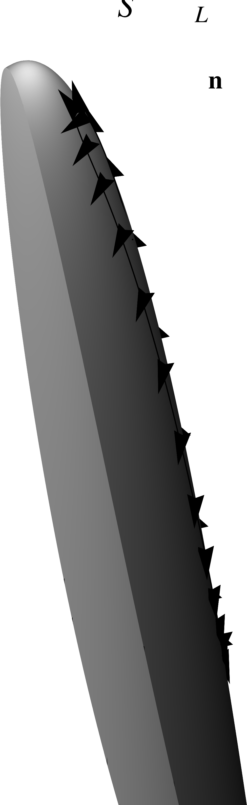
Remarkably, the tensor formulation of the divergence theorem remains completely intact for curved domains. Suppose that $S$ is a curved domain with a contour boundary $L$ and let $n^{\alpha}$ be the surface components of its outward geodesic normal $\mathbf{n}$. Then, for a surface tensor $T^{\alpha}$, the divergence theorem reads The curved form of the divergence theorem also remains valid for tensors with vector elements, i.e. Note that one of the essential aspects of the divergence theorem is its invariant nature. Indeed, all elements of the theorem are invariant objects that can, at least conceptually, be evaluated without the use of a coordinate system.

Crucially, the scalar forms of the divergence theorem do not include any elements specific to Euclidean spaces. Thus, the statements of the theorem remain meaningful -- and, perhaps more importantly, correct -- in the more general Riemannian spaces and generalize to arbitrary dimension. Note that while the use of the letters $S$ and $L$, which we have typically used for two-dimensional domains and their one-dimensional contour boundaries, suggests that the equation is two-dimensional, it can actually be validly interpreted for a domain $S$ of any dimension $n$ with an $\left( n-1\right)$-dimensional boundary $L$. In this arbitrary-dimensional Riemannian interpretation, there is in fact no difference between the above form and which can be considered a special case of the more general Riemannian interpretation.

In the upcoming investigations, we will strike a compromise between the Euclidean and Riemannian perspectives. For the sake of geometric intuition, we will discuss the specific case of a curved two-dimensional surface $S$ in a Euclidean space. However, we will restrict ourselves to analytical arguments that remain valid in the more general Riemannian spaces.

Before we turn our attention to the derivation of the divergence theorem, let us take a look at a few of its striking theoretical applications in a Euclidean space

For any Euclidean domain $\Omega$, the integral of the unit normal $\mathbf{N}$ over its boundary $S$ vanishes, i.e. The demonstration of this relationship by the divergence theorem is entirely straightforward. Since the integral in question can be written in component form as an application of the divergence theorem yields Now, thanks to the metrinilic property of the covariant derivative with respect to the covariant basis $\mathbf{Z}_{i}$, i.e. we find that as we set out to show. Finally, we note that this integral may be interpreted as the net force on the body occupying the domain $\Omega$ from a uniform pressure field. The fact that the integral vanishes is consistent with our experience that a free body placed in a uniform pressure field remains at equilibrium.

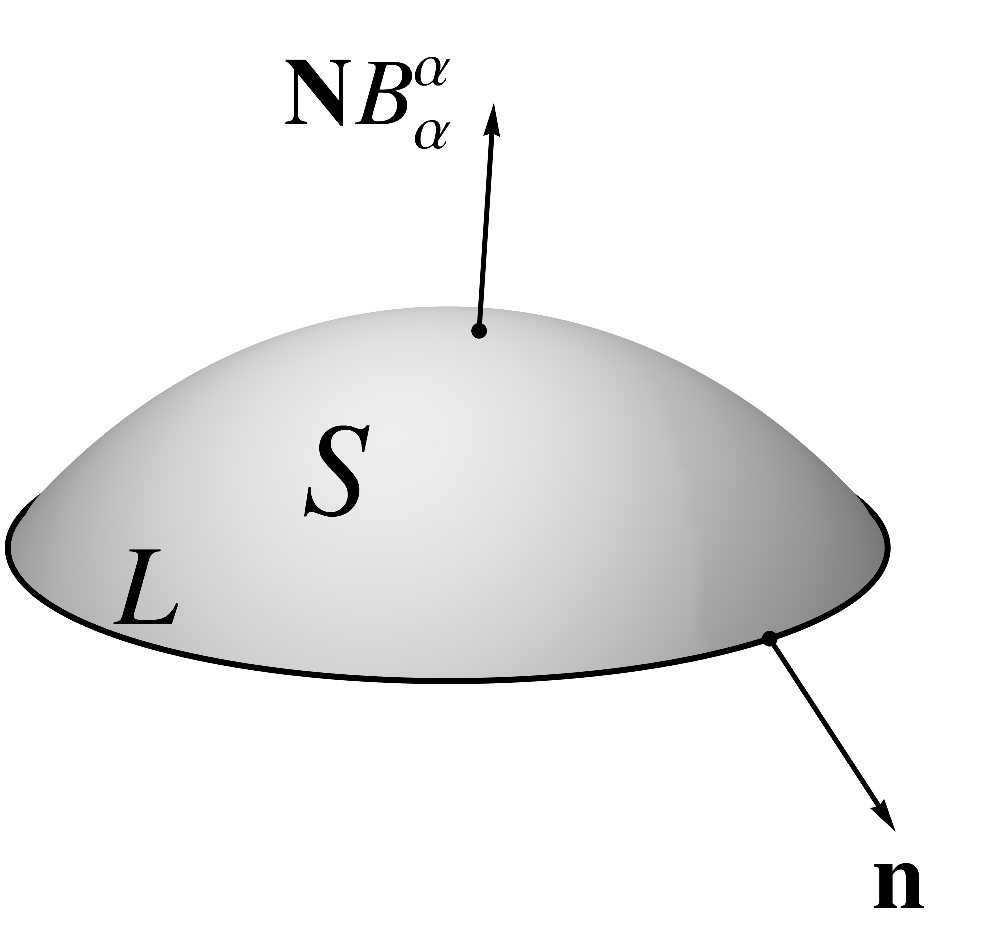
For an application of the divergence theorem to a curved domain, let us now consider a similar integral of the curvature normal $\mathbf{N}B_{\alpha}^{\alpha}$ over a surface patch $S$ with boundary $L$. Under the Laplace model of capillary forces, this integral may be interpreted as the net force of surface tension acting upon a soap film represented by the curved surface $S$. Since, in our experience, the center of mass of a soap bubble does not experience acceleration under the influence of surface tension, we expect this integral to also equal zero for a closed surface $S$.

Recall that the combination $\mathbf{N}B_{\alpha}^{\alpha}$ equals the surface Laplacian of the position vector $\mathbf{R}$, i.e. or, equivalently, the divergence of the surface contravariant basis $\mathbf{S}^{\alpha}$, i.e. Therefore, by the divergence theorem, we have Since the combination $n_{\alpha}\mathbf{S}^{\alpha}$ represents the outward geodesic normal $\mathbf{n}$, we have In words, the integral of the curvature normal $\mathbf{N}B_{\alpha}^{\alpha}$ over a surface patch equals the integral of the outward geodesic normal $\mathbf{n}$ over the contour of the patch.

By all accounts, this relationship makes intuitive geometric sense, especially over a small patch: the more curved is the patch, the more the geodesic normals at its boundary point in a consistent direction. If the patch is flat, i.e. $B_{\alpha}^{\alpha}=0$, then the contour integral vanishes, i.e. which is precisely the two-dimensional version of the Euclidean formula in the previous example.

Furthermore, we observe that the curvature normal $\mathbf{N}B_{\alpha }^{\alpha}$ at a given point $P$ is given by the limit where each integral is calculated over a patch $S$ that is shrinking to the point $P$ in a regular manner. Dotting both sides with $\mathbf{N}$ gives an explicit limit for the mean curvature $B_{\alpha}^{\alpha}$, i.e.

Finally, note that when the patch $S$ represents a closed surface, i.e. there is no boundary, the formula implies that the integral of the curvature normal $\mathbf{N}B_{\alpha }^{\alpha}$ vanishes, i.e. as we expected.

The relationships discussed above have interesting "companion" formulas where the integrand is dot multiplied by the position vector field $\mathbf{R}$. All of these formulas also follow from the divergence theorem and their proofs are left as exercises.

For a closed surface $S$, the volume $V$ of the enclosed domain $\Omega$ is given in terms of the surface integral of $\mathbf{R}\cdot\mathbf{N}$ by the formula where $n$ is the dimension of the ambient space.

Similarly, the surface integral of $\mathbf{R}\cdot\mathbf{N}B_{\alpha }^{\alpha}$ over $S$ yields its area $A$ according to the formula For a non-closed patch $S$ with boundary $L$, the analogous formula reads (Note that despite the use of the same letter, there is no relation between the dimension $n$ of the ambient space and the geodesic normal $\mathbf{n}$.)

What happens when the mean curvature $B_{\alpha}^{\alpha}$ in the above integrals is replaced with Gaussian curvature $K$? It turns out that for a closed two-dimensional surface $S$, the integral of $\mathbf{N}K$ vanishes, i.e. Meanwhile, the companion formula reads

In Chapter TBD of Introduction Tensor Calculus we described the concept of a geometric integral. Whether it is a volume integral a surface integral or a line integral a geometric integral represents the additive total of an invariant quantity over a geometric domain. In the same Chapter, we described the evaluation of geometric integrals by a limiting procedure that involves subdividing the domain into ever small pieces and adding up the individual infinitesimal contributions. The main takeaway of the procedure is that, at least theoretically, geometric integrals can be evaluated by invariant means without a reference to a coordinate system.

On the other hand, for many practical as well as theoretical reasons, geometric integrals must be converted into arithmetic integrals which can be evaluated by the techniques of ordinary Calculus, such as the Fundamental Theorem of Calculus, or other means, such as numerical computation. Naturally, translation to an arithmetic integral becomes possible once the domain is referred to a coordinate system. As we stated in Chapter TBD of Introduction to Tensor Calculus, the volume integral corresponds to the arithmetic integral where $\sqrt{Z}$ is the volume element, the limits of integration reflect the domain, and it is further stipulated that each lower limit is less than the corresponding limit, i.e. Correspondingly, for surface and line integrals, we have and with the same stipulation regarding the integration limits. In order for these conversions to be valid, however, it must be demonstrated that the arithmetic integrals are invariant with respect to coordinate changes. This will be one of the tasks accomplished in the next Section.

For an example of conversion from a geometric to an arithmetic integral, consider the classical calculation of the volume $V$ of a sphere of radius $R$. As a geometric integral, $V$ is given by the formula In Cartesian coordinates $x,y,z$, the volume element $\sqrt{Z}$ is given by and therefore the corresponding arithmetic integral reads In spherical coordinates $r,\theta,\varphi$, on the other hand, the expression for the volume element $\sqrt{Z}$ is and therefore the corresponding arithmetic integral reads Both integrals evaluate to consistent with the expected invariance of the arithmetic integral with respect to coordinate changes. The latter integral, however, is much easier to evaluate which illustrates the benefit of choosing a coordinate system that is suited to a specific task.

The argument presented in this Section relies on the change-of-variables theorem from Multivariable Calculus. Our goal is to show that the two arithmetic integrals and constructed according to the algorithm described above for two alternative coordinate systems $Z^{i}$ and $Z^{i^{\prime}}$, are equal.

Recall that according to the change-of-variables theorem, the integral for a function $g\left( Z\right)$ in coordinates $Z^{i}$ can be transformed to an equivalent integral in coordinates $Z^{i^{\prime}}$ by implementing three changes: 1. substituting the change of variables $Z^{i}\left( Z^{\prime}\right)$ for the variables in the function $g\left( Z\right)$, 2. introducing a factor of $\det^{-1}J$, where $J$ is the matrix representing the Jacobian $J_{i^{\prime}}^{i}$, and 3. appropriately adjusting the limits of integration. These three steps are summarized by the formula When we apply this formula to the integral we find Of course, the composition $F\left( Z\left( Z^{\prime}\right) \right)$ is precisely $F\left( Z^{\prime}\right)$, i.e. the field $F$ as a function of the primed coordinates $Z^{i^{\prime}}$. Also, recall from Section TBD of Introduction to Tensor Calculus that the volume element $\sqrt{Z}$ transforms as a relative invariant of weight $-1$, i.e. Thus, the combination $F\left( Z\left( Z^{\prime}\right) \right) \sqrt {Z}J^{-1}$ equals $F\left( Z^{\prime}\right) \sqrt{Z^{\prime}}$ and we have as we set out to show.

We will prove the divergence theorem in two steps. In this Section, we will demonstrate the "arithmetic" version of the divergence theorem for a tensor field $T^{\alpha}$ over a planar domain $\bar{S}$ with boundary $\bar{L}$ referred to Cartesian coordinates $x$ and $y$. Although the domain $\bar{S}$ and its boundary $\bar{L}$ need not be the arithmetic representation of some curved domain $S$ with boundary $L$, we chose to use the bar accent to highlight the Cartesian nature of the present discussion. Note that and Therefore, in the unpacked form, the arithmetic divergence theorem reads

Once we prove the arithmetic version of the divergence theorem, we will prove the general divergence theorem by reducing it to its arithmetic version

In Chapter TBD of Introduction to Tensor Calculus, we defined the arithmetic space associated with a Riemannian space as a Cartesian visualization of the coordinate system in a Euclidean space. For instance, for a two-dimensional surface referred to surface coordinates $S^{\alpha}$, the arithmetic space imagines the coordinates $S^{1}$ and $S^{2}$ as Cartesian coordinates in the plane.

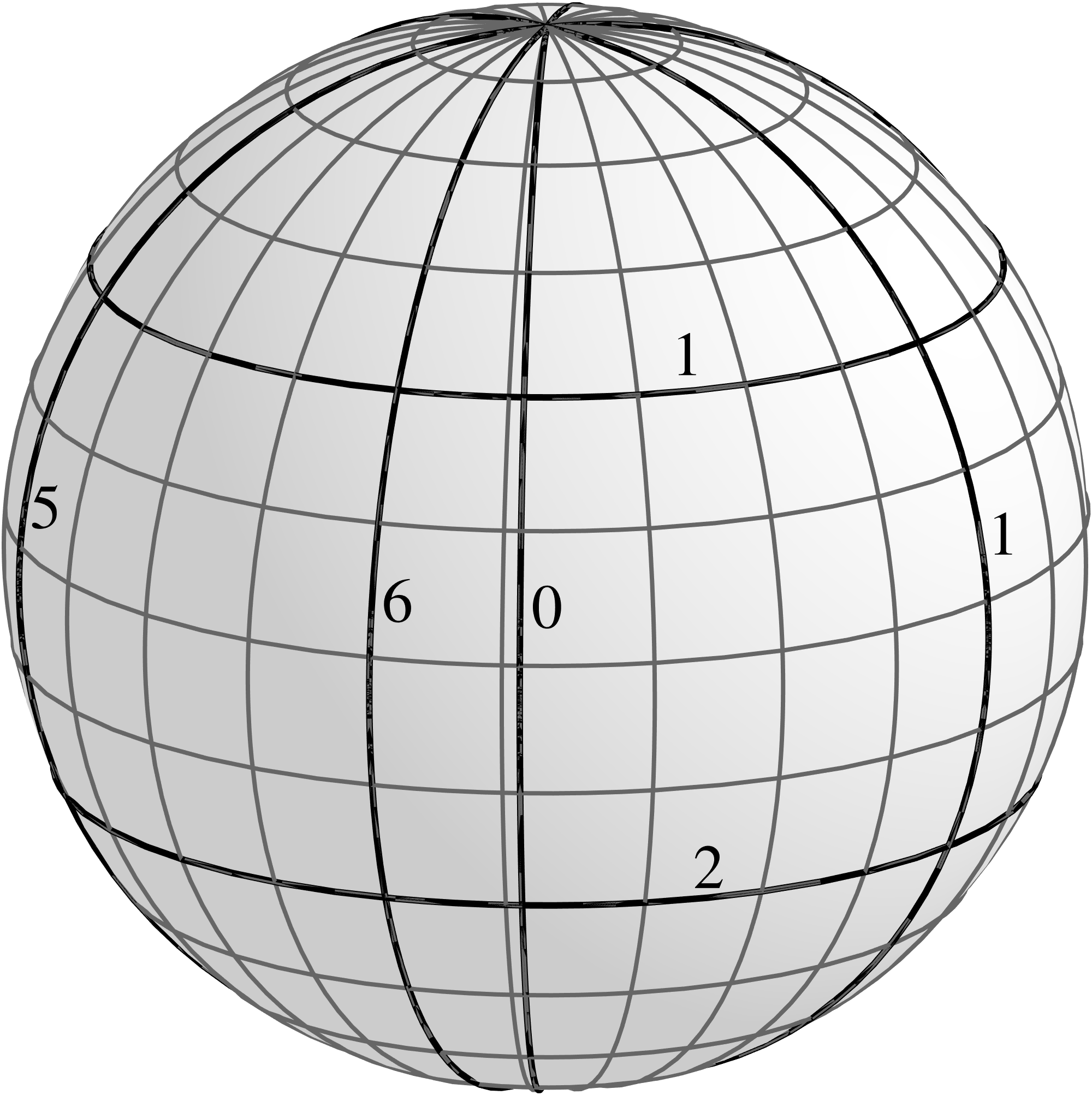
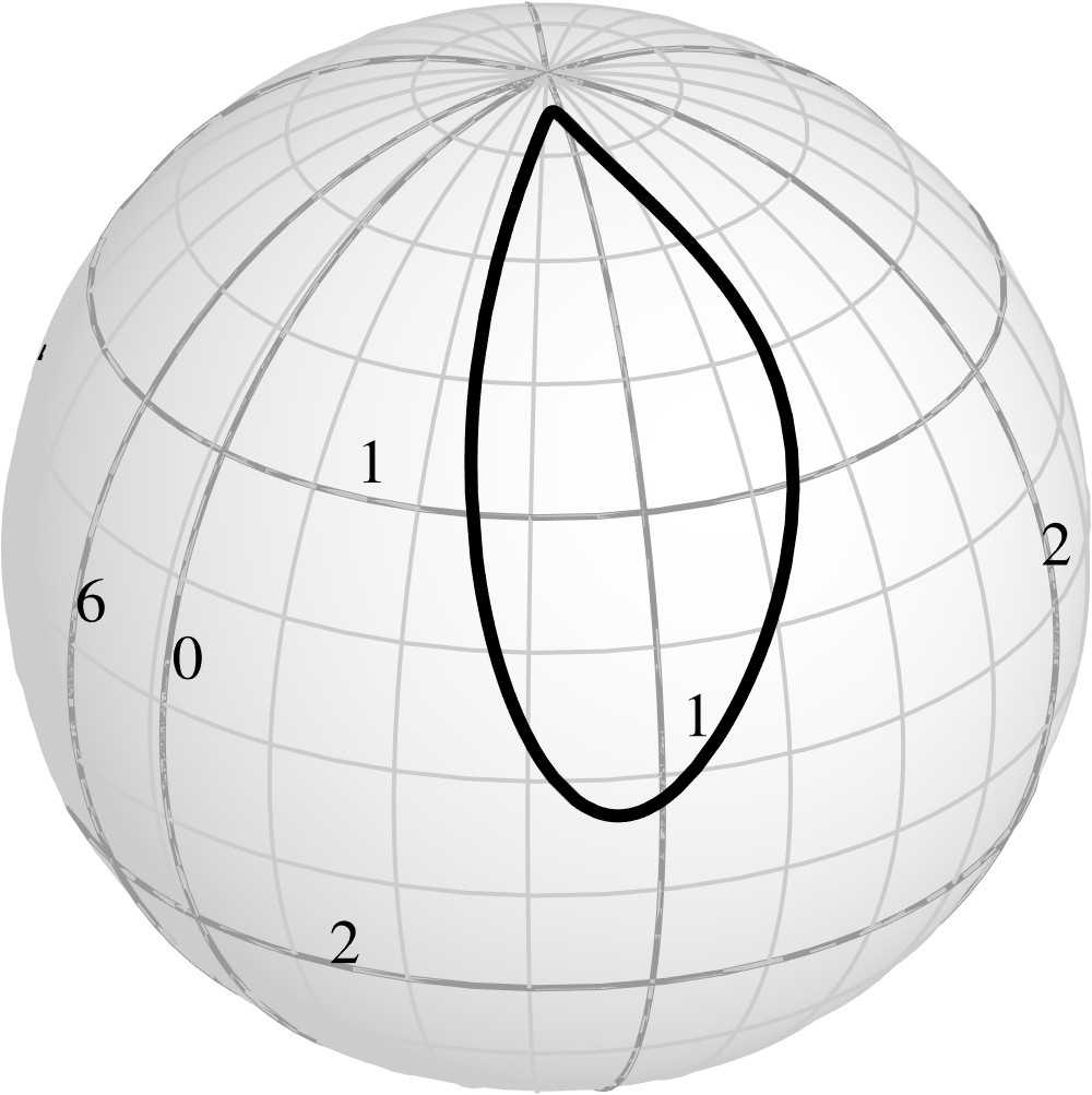
For a specific example, consider a sphere of radius $R$ referred to the standard spherical coordinates $\theta$ and $\varphi$. The corresponding arithmetic space occupies a $\pi\times2\pi$ rectangle in the plane, as illustrated in the following figure. Furthermore, to any surface curve described by the equations there corresponds a curve in the arithmetic space described by the same equations. The following figure shows an example of a curve on a sphere along with its arithmetic counterpart. Entirely unsurprisingly, the two shapes are completely different.

In the upcoming demonstration of the divergence theorem, we will use a generic curved patch illustrated in the following figure along with its arithmetic representation.

The fascinating aspect of the argument that we are about to present is that the geometry of the arithmetic representation will take on central relevance. We will use the bar accent above the symbol to denote the geometric objects in the arithmetic space. Thus, the domain $S$ corresponds to the arithmetic domain $\bar{S}$ and its boundary $L$ corresponds to the curve $\bar{L}$. The shape of the curve $\bar{L}$ in the arithmetic space will give rise to the normal field $\mathbf{\bar{n}}$. And although we are about to show that the components $n^{\alpha}$ and $\bar{n}^{\alpha}$ are related, there is no reason whatsoever to expect that $n^{\alpha}=\bar{n}^{\alpha}$.

While the curves $L$ and $\bar{L}$ live in completely different spaces, they are, by construction, described by the same equations Therefore, their respective shift tensors are identical as well.

On the other hand, the area elements $\sqrt{S}$ and $\sqrt{\bar{S}}$ are different, as are the line elements $\sqrt{L}$ and $\sqrt{\bar{L}}$. Note that since the coordinates $S^{1}$ and $S^{2}$ play the role of Cartesian coordinates in arithmetic space, we have

We are now in a position to relate the components $n^{\alpha}$ of the geodesic normal $\mathbf{n}$ to the original curve $L$ and the components $\bar {n}^{\alpha}$ of the normal $\mathbf{\bar{n}}$ to the arithmetic curve $\bar{L}$. Recall that these components are given by the equations and where we once again point out that the shift tensor $S_{\Phi}^{\alpha}$ is the same for both curves. Expressing the Levi-Civita symbols in terms of the corresponding permutation systems $e_{\alpha\beta}$ and $e^{\Phi}$, we find Thus, and therefore Finally, since we arrive at the formula which will be used below to bridge the divergence theorem to its arithmetic analogue.

The Fundamental Theorem of Calculus tells us that the operations of integration and differentiation are the inverses of each other. The equation can be seen as the "integral of the derivative" form of the theorem. To obtain the "derivative of the integral form", allow the upper limit of the integral to vary, i.e. and differentiate both sides with respect to $x$, i.e. It is this "derivative of the integral" form, along with its straightforward extensions we are about to describe, that will be of greater to use to us in our current discussion.

First, allow the upper limit to be a general function $y\left( x\right)$ of $x$. Then, by the chain rule, we have It is left as an exercise to show that the corresponding formula for a variable lower limit reads Finally, suppose that the variable $x$ also appears as a parameter in the integrand, i.e. Then the integral is once again a function of $x$ and can therefore be differentiated with respect to $x$. Since an integral is essentially a sum, it is not surprising that in order to differentiate the integral we must differentiate the integrand, i.e.

In summary, let us combine the three possible ways in which the integral can depend on the variable $x$ in a single equation, i.e.

Finally, our proof of the arithmetic divergence theorem will require expressions for the length element $L$ and the normal components $n^{a}$ for a curve given by an explicit function in Cartesian coordinates. Recall the equations from Chapter 4 where we switched from $S$ to $\bar{L}$ and from $N^{i}$ to $\bar{n}^{\alpha}$ to fit the current context. Note that the components of $\bar{n}^{\alpha}$ were chosen so that they correspond to the "upward" normal.

Given the expression for $\bar{L}$, the line integral in arithmetic form reads

Our argument will be limited to two-dimensional domains that correspond to a region between two functions $y_{1}\left( x\right)$ and $y_{2}\left( x\right)$, as illustrated in the following figure. Note that along the top potion of the curve, the exterior normal points up, while along the bottom portion of the curve, the exterior normal points down. In the previous Section, we gave an expression for the "upward" normal. However, on the bottom portion of the curve described by $y_{1}\left( x\right)$, the outward normal points downwards and we must therefore adjust our expressions. We have

Denote the elements of the tensor field $T^{\alpha}$ by $G$ and $H$, i.e. Then the divergence $\nabla_{\alpha}T^{\alpha}$ of $T^{\alpha}$ is given by and the volume integral of $\nabla_{\alpha}T^{\alpha}$ is given by the repeated integral Breaking the repeated integral on the right up into two, we have

We will now analyze each repeated integral individually. However, for both integrals, the key step involves an application of the Fundamental Theorem of Calculus to the "inner" integral, i.e. in the case of $I_{1}$ and in the case of $I_{2}$. For each fixed value of $x$, the integration in the inner integrals takes place along the vertical interval from $y_{1}\left( x\right)$ to $y_{2}\left( x\right)$ and reduces the integral to the difference of two values corresponding to the two ends of the integration intervals. As a result, the "outer" integrals represent sums of combinations involving the boundary values of $G$ and $H$ as well as the derivatives of $y_{1}^{\prime}\left( x\right)$ and $y_{2}^{\prime}\left( x\right)$ and thus can eventually be converted into line integrals over the boundary $\bar{L}$. This shows how the Fundamental Theorem of Calculus reduces a domain integral to a boundary integral and demonstrates why the divergence theorem may be considered a direct consequence of the Fundamental Theorem of Calculus.

We begin with the integral Consider the inner integral and notice that this integral can be related to with the help of the extension of the Fundamental Theorem of Calculus derived earlier and captured by the equation Substituting $G\left( x,y\right)$ for $f\left( x,\xi\right)$, we find Thus, Now, recall that and note that, by the Fundamental Theorem of Calculus, and each integral on the right vanishes since and therefore the lower and the upper limits for each integral coincide.

Consequently, the final expression for $I_{1}$ reads We will now turn our attention to the integral $I_{2}$.

The analysis of is far simpler than that of $I_{1}$ since the inner integral is tailor-made for an application of the Fundamental Theorem of Calculus. Indeed, Therefore,

Combining the two integrals and grouping together the terms involving $y_{1}\left( x\right)$ and those involving $y_{2}\left( x\right)$, we find We can rewrite the integrand of each integral as a dot product, i.e. Note the objects are not quite the components $\bar{n}^{\alpha}$ of the normal along $\bar {L}_{1}$ and $\bar{L}_{2}$, since they are missing factors of Similarly, the two integrals above do not quite represent line integrals over $\bar{L}_{1}$ and $\bar{L}_{2}$ since they are missing the requisite factors of Clearly, the missing factors are the reciprocals of each other and therefore both problems can be easily remedied at the same time by writing the integrals in the form We now readily recognize the first integrand as $\int_{\bar{L}_{1}}\bar {n}_{\alpha}T^{\alpha}d\bar{L}$ and the second integral as $\int_{\bar{L}_{2} }\bar{n}_{\alpha}T^{\alpha}d\bar{L}$. Thus, as we set out to prove.

We will now use the "arithmetic" divergence theorem to prove the general formulation for a curved domain $S$ with boundary $L$.

As step one, convert the volume integral to a repeated arithmetic integral, i.e. Note that we have omitted the limits of integration for the repeated integrals and it is understood that the limits are chosen in such a way as to correctly describe the domain $S$.

Recall that, according to the Voss-Weyl formula Thus the combination $\nabla_{\alpha}T^{\alpha}\sqrt{S}$ is given by and therefore Notice that the integral on the right equals the integral since the "missing" factor of $\sqrt{\bar{S}}$ equals $1$. Thus, by the arithmetic divergence theorem that we have just demonstrated, we have